DOI: 10.1534/genetics.110.116426
Graph-Based Data Selection for the Construction
of Genomic Prediction Models
Steven Maenhout,*
,1Bernard De Baets
§and Geert Haesaert*
*Department of Biosciences and Landscape Architecture, University College Ghent, B-9000 Gent, Belgium,§Department of Applied Mathematics, Biometrics and Process Control, Ghent University, B-9000 Gent, Belgium
Manuscript received March 8, 2010 Accepted for publication May 11, 2010
ABSTRACT
Efficient genomic selection in animals or crops requires the accurate prediction of the agronomic performance of individuals from their high-density molecular marker profiles. Using a training data set that contains the genotypic and phenotypic information of a large number of individuals, each marker or marker allele is associated with an estimated effect on the trait under study. These estimated marker effects are subsequently used for making predictions on individuals for which no phenotypic records are available. As most plant and animal breeding programs are currently still phenotype driven, the continuously expanding collection of phenotypic records can only be used to construct a genomic prediction model if a dense molecular marker fingerprint is available for each phenotyped individual. However, as the genotyping budget is generally limited, the genomic prediction model can only be constructed using a subset of the tested individuals and possibly a genome-covering subset of the molecular markers. In this article, we demonstrate how an optimal selection of individuals can be made with respect to the quality of their available phenotypic data. We also demonstrate how the total number of molecular markers can be reduced while a maximum genome coverage is ensured. The third selection problem we tackle is specific to the construction of a genomic prediction model for a hybrid breeding program where only molecular marker fingerprints of the homozygous parents are available. We show how to identify the set of parental inbred lines of a predefined size that has produced the highest number of progeny. These three selection approaches are put into practice in a simulation study where we demonstrate how the trade-off between sample size and sample quality affects the prediction accuracy of genomic prediction models for hybrid maize.
D
ESPITE the numerous studies devoted to molec-ular marker-based breeding, the genetic progress of most complex traits in today’s plant and animal breeding programs still heavily relies on phenotypic selection. Most breeding companies have established dedicated databases that store the vast number of phenotypic records that are being routinely collected throughout the course of their breeding programs. These phenotypic records are, however, gradually being complemented by various types of molecular marker scores and it is to be expected that effective marker-based selection schemes will eventually allow current phenotyping efforts to be reduced (Bernardo 2008;Hayes et al. 2009). The available marker and
pheno-typic databases already allow for the construction and validation of marker-based selection schemes. Mining the phenotypic databases of a breeding company is, however, quite different from analyzing the data that is generated by a carefully designed experiment. Genetic evaluation data is often severely unbalanced as elite
individuals are usually tested many times on their way to becoming a commercial variety or sire, while less per-forming individuals are often disregarded after a single trial. Furthermore, the different phenotypic evaluation trials are separated in time and space and as such, sub-jected to different environmental conditions. Therefore, ranking the performance of individuals that were evalu-ated in different phenotypic trials is usually a nontrivial task.
Animal breeders are well experienced when it comes to handling unbalanced genetic evaluation data. The best linear unbiased predictor or BLUP approach (Henderson 1975) presented a major breakthrough
in this respect, especially when combined with restricted maximum-likelihood or REML estimation of the need-ed variance components (Pattersonand Thompson
1971). Somewhat later on, this linear mixed modeling approach was also adopted by plant breeders as thede facto standard for handling unbalanced phenotypic data. The more recent developments in genomic selection (Bernardo 1995; Meuwissen et al. 2001;
GianolaandvanKaam2008) and marker-trait
associ-ation studies (Yuet al. 2006) are, at least partially,
BLUP-based and are therefore, in theory, perfectly suited for
1Corresponding author : Department of Biosciences and Landscape
Architecture, University College Ghent, Voskenslaan 270, B-9000 Gent, Belgium. E-mail: [email protected]
mining the large marker and phenotypic databases that back each breeding program. In practice, however, the unbalancedness of the available genetic evaluation data often reduces its total information content and the construction of a marker-based selection model is limited to a more balanced subset of the data.
As phenotypic data are available, genotyping costs limit the total number of individuals that can be includ-ed in the construction of a genomic princlud-ediction model. The best results will be obtained by selecting a subset of individuals for which the phenotypic evaluation data exhibits the least amount of unbalancedness. In this article we demonstrate how this phenotypic subset selection problem can be translated into a standard graph theory problem that can be solved with exact algorithms or less-time-consuming heuristics.
In most plant and animal species, the number of available molecular markers is rapidly increasing, while the genotyping cost per marker is decreasing. Neverthe-less, as budgets are always limited, genotyping all map-ped markers for a small number of individuals might be less efficient than genotyping a restricted set of well-chosen markers on a wider set of individuals. One should therefore be able to select a subset of molecular markers that covers the entire genome as uniformly as possible. We demonstrate how this marker selection problem can also be translated into a well-known graph theory problem that has an exact solution.
The third problem we tackle by means of graph theory is more specific to hybrid breeding programs where the parental individuals are nearly or completely homozy-gous. This implies that we can deduce the molecular marker fingerprint of a hybrid individual from the mark-er scores of its parents. As the phenotypic data are collected on the hybrids, genotyping costs can be re-duced by selecting a subset of parental inbreds that have produced the maximum number of genetically distinct offspring among themselves. Obviously, the phenotypic data on these offspring should be as balanced as possible. Besides solving the above-mentioned selection prob-lems by means of graph theory algorithms, we demon-strate their use in a simulation study that allows us to determine the optimum trade-off between the number of individuals and the size of the genotyped molecular marker fingerprint for predicting the phenotypic per-formance of hybrid maize by means ofe-insensitive sup-port vector machine regression (e-SVR) (Maenhout et al. 2007, 2008, 2010) and best linear prediction (BLP) (Bernardo1994, 1995, 1996).
SELECTING INDIVIDUALS FROM UNBALANCED PHENOTYPIC EVALUATION DATA
In most plant or animal breeding programs, all phenotypic measurements that were recorded during genetic evaluation trials are stored for future reference. The all-encompassing experimental design that
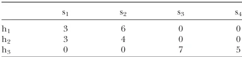
gener-ated the data is likely to be very unbalanced. The most extreme case of an unbalanced design is a disconnected design. Table 1 gives an example of a disconnected sire evaluation design taken from Kennedy and Trus
(1993). The breeding values of four sires are evaluated by measuring the performance of their offspring in three different herds. Sires having offspring in different herds provide vertical connections between herds while herds containing offspring of different sires provide horizontal connections. In a perfectly balanced design, each sire would have the same number of offspring tested in each herd. In the presented scenario, however, sires s1and s2are disconnected from sires s3and s4as there is no possible path between these groups. This means that if we analyze the phenotypic data from this design with an ordinary least-squares model, contrasts involving sires that belong to the disconnected groups would be inestimable. However, if we fit a linear mixed model to the data in which we assume herds as fixed and sires as random effects, contrasts involving sire BLUPs belonging to these disconnected groups are perfectly estimable.
Ignoring connectivity issues by treating sire effects as random variables is, however, not without consequence. This approach implicitly assumes that all evaluated individuals originate from the same population and as such have the same breeding value expectation. This assumption is generally not valid in animal breeding programs as the better sires are usually evaluated in the better herds (Foulleyet al. 1990). A similar
stratifica-tion can be observed in genetic evaluastratifica-tion trials performed by plant breeders where late and therefore higher-yielding individuals are generally tested in geo-graphical regions with longer growing seasons. As a consequence, BLUP-based genomic selection routines will be less efficient, while marker-trait association studies will suffer from increased false positive rates and reduced power. A very unbalanced but nevertheless connected design will also reduce the effectiveness of marker-based selection approaches as the prediction error variance of the estimated breeding values in-creases substantially. Furthermore, the estimated breed-ing values will be regressed toward the mean and will not account for the true genetic trend.
TABLE 1
Example of a disconnected sire3herd design taken from KENNEDYand TRUS(1993)
s1 s2 s3 s4
h1 3 6 0 0
h2 3 4 0 0
h3 0 0 7 5
We can assume that the available data set contains unbalanced phenotypic measurements ontindividuals, wheretis generally a very large number. The available phenotypic data allow the breeder to try out one or more of the more recent BLUP-based genomic selection approaches without setting up dedicated trials. Given his financial limit for genotyping, he wants to select exactlypindividuals from this data set. The selection of p individuals should be optimal in the sense that the precision of the BLUPs of thepbreeding values that are obtained from a linear mixed model analysis of the full set of phenotypic records is superior to the precision of any other set of BLUPs with cardinalityp. This optimality criterion requires a measure of precision of a subset of BLUPs obtained from a linear mixed model analysis. To introduce this criterion, we will make the general assumption that the applied linear mixed model takes the form
y¼Xb1Zu1e; ð1Þ
where y is a column vector containing n phenotypic measurements on thetindividuals.bis a vector of fixed nuisance effects like trial, herd, and replication effects anduis a vector containing random genetic effects for each of thet individuals. For ease of explanation, we assume thatucontains onlytbreeding values, but the presented approach can easily be generalized to cases where u is made up from general combining abilities (GCA) and specific combining abilities (SCA) and possibly the different levels of various genotype-by-environment (G 3 E) interaction factors. Vector e contains n random residuals. Matrices X and Z link the appropriate phenotypic records to the effects inb andu, respectively. Furthermore we assume that we can represent the variance ofuandeas
Var u e ¼
G 0
0 R
:
Gcan contain an assumed covariance structure for thetindividuals, typically a scaled numerator relation-ship matrix calculated from available pedigree or mark-er data. It is, howevmark-er, important to realize that fitting a covariance between breeding values allows the BLUPs from individuals that have little phenotypic information themselves, to borrow strength from phenotypic re-cords on closely related individuals. As a result, thep individuals with highest BLUP precision will most likely be close relatives, which is detrimental for the general-izing capabilities of the marker-based selection model. If we want the selection of p individuals to rely com-pletely on the amount of information and the structure (balancedness) of their phenotypic records,Gshould be a scaled identity matrix. Once thepindividuals have been selected, a pedigree or marker-based covariance structure can be incorporated inGfor the construction of the actual marker-based prediction model. The
covariance structure of the residuals in matrix R can contain heterogeneous variances for the different pro-duction environments or, in case that data originates from actual field trials, spatial information like row or column correlations. The BLUPs in vectoruare obtained by solving the mixed model equations (Henderson
1984)
X9R1X X9R1Z Z9R1X Z9R1Z1G1
ˆ
b ˆ
u ¼
X9R1y Z9R1y
:
The inverse of the coefficient matrix allows to obtain the prediction error variance (PEV) matrix of vectoruˆas
X9R1X X9R1Z Z9R1X Z9R1Z1G1
1
¼ C11 C12
C21 C22
;
where
PEVðˆuÞ ¼VarðˆuuÞ ¼C22:
A logical choice of measure to express the precision of a selection ofpBLUPs from thetcandidates in vectoruˆ would be some function of thep3pprincipal submatrix Cp22, obtained by removing the rows and columns ofC22 that pertain to individuals that are not in that particular selection. As a good design is strongly associated with the precision of pairwise contrasts (BuenoFilhoand
Gilmour 2003), we use the lowest precision of all
possible pairwise contrast vectors between thepselected individuals as optimization criterion. A pairwise contrast vector qij for the individuals i and j is a vector where qiij¼1 andq
ij
i ¼ 1, while all other elements of qij are zeros. Laloe´ (1993) and Laloe´ et al. (1996) propose expressing the precision of a linear contrast vector q by means of the generalized coefficient of determination (CD), which is defined as
CDðqÞ ¼q9ðGC22Þq q9Gq ;
where CDðqÞalways lies within the unit interval. They indicate that CDðqÞ can be obtained as a weighted average of the t – 1 nonzero eigenvalues mi of the generalized eigenvalue problem
ððGC22Þ miGÞvi¼0; ð2Þ
as
CDðqÞ ¼
Pt i¼2ai2mi
Pt i¼2ai2
; ð3Þ
where ai2 is the weight for eigenvalue i and the first eigenvaluem1always equals zero as a consequence of the well-known summation constraint 19G1uˆ (see, e.g., Foulleyet al. 1990). Each linear contrast vectorqcan
q¼X t
i¼2
aivi:
In fact, all linear contrast vectors that are estimable in the least-squares sense are linear combinations of the eigenvectors vi of Equation 2 that are associated to nonzero eigenvaluesmi, while those contrasts that are not estimable in a least-squares sense are linear combi-nations of eigenvectors for which at least one associated eigenvalue is zero. This implies that the CD of a pairwise contrast vector involving two individuals that were evaluated in two disconnected groups does not neces-sarily become zero as several eigenvaluesmiin Equation 3 might be nonzero. This might bias the selection procedure to favor a disconnected set of individuals with a high information content (i.e.,a high level of replica-tion) instead of a connected set of individuals with low information content. To avoid this situation, the CD of pairwise contrast vectors between disconnected individ-uals should be forced to zero. In case Equation 1 represents a simplified animal model where G¼Is2 g andR¼Is2
e, disconnected pairs of individuals can be easily identified by examining the block diagonal struc-ture of the PEV matrixC22as explained in Appendix A. In Appendix B we show how disconnected pairs of individuals can be identified by means of the transitive closure of the adjacency matrix of thetindividuals.
Now that we have the corrected CD for each of the pðp1Þ=2 pairwise contrast vectors, we can represent the t individuals as vertices (also called nodes) of a weighted complete graph where the edge between individualiand individualjcarries the weight CDðqijÞ, expressing the precision of the pairwise contrast as a number between zero and one. We need to select exactlyp vertices such that the minimum edge weight in the selected subgraph is maximized. This problem is equivalent to the ‘‘discretep-dispersion problem’’ from the field of graph theory. This problem setting is encountered when locating facilities that should not be clustered in one location, like nuclear plants or franchises belonging to the same fast-food chain. This problem is nondeterministic polynomial-time (NP)-hard even when the distance matrix satisfies the triangle inequality. Erkut(1990) describes two exact algorithms
that are based on a branch and bound strategy and compares 10 different heuristics (Erkutet al. 1994). An
interesting solution lies in the connection between the discretep-dispersion problem and the maximum clique problem. A clique in a graph is a set of pairwise adjacent vertices or, in other words, a complete subgraph. The corresponding optimization problem, the maximum clique problem, is to find the largest clique in a graph. This problem is also NP-hard (Carraghanand P arda-los 1990). The idea is to decompose the discrete p
-dispersion problem in a number of maximum clique problems by assigning different values to the minimum
required contrast precision CDmin. Initially, CDminis low (e.g., CDmin ¼ 0.1) and we define a graph G9(V, E9), where the edges of the original graph Gare removed when their edge weight is smaller than CDmin. This implies that there will be no edges between discon-nected pairs of individuals in the derived graph as these edge weights have been set to zero by the CD correction procedure. Solving the maximum clique problem in G9(V,E9) allows us to identify a complete subgraph for which all edge weights are guaranteed to be greater than CDmin. The number of vertices in this complete subgraph is generally smaller thantbut greater thanp. By repeating this procedure with increasing values of CDminone can make a trade-off between sample size and sample quality as demonstrated in Figure 1 for a representative sample of sizet¼4236 individuals for which genetic evaluation data were recorded as part of the grain maize breeding program of the private company RAGT R2n. Each dot represents the largest possible selection of individuals where CDminranges from 0 to 0.97. The data used in this example are connected as there is no sudden drop in the number of individuals when CDminis raised from 0.0 to 0.1. In general, the surface below the curve represents a measure of data quality. If one is interested only in obtaining the optimal selection of exactlyp individuals from a set of t candidates, one can implement the described maximum clique-based procedure in a binary search.
obtained. Several exact algorithms and heuristics have been published, but comparing these is often difficult as the dimensions and densities of the provided example graphs as well as computational platforms tend to differ between articles. The exact algorithm of Carraghan
and Pardalos (1990) is, however, considered as the
basis for most later algorithms. Although the efficiency of this algorithm has been superseded by that of more recent developments (O¨ sterga˚ rd 2002; Tomita and
Seki2003), its easy implementation often makes it the
method of choice. If the available run-time is limited, a time-constrained heuristic like the reactive local search approach presented by Battiti and Protasi (2001)
might be more appropriate. Bomzeet al. (1999) give an
overview of several other heuristic approaches found in literature, in particular greedy construction and sto-chastic local search, including simulated annealing, genetic algorithms, and tabu search.
SELECTING MARKERS FROM A DENSE MOLECULAR MARKER FINGERPRINT
The construction of a genomic prediction model requires genotypic information on each of the p selected individuals. Generally it is assumed that a good prediction accuracy can only be achieved by maximizing the genome coverage, which implies genotyping a large number of molecular markers. This approach seems particularly attractive as genotyping costs are decreasing rapidly. However, as shown by Maenhoutet al. (2010),
the relation between the number of genotyped markers and the obtained prediction accuracy seems to be subject to the law of diminishing marginal returns. This means that it might be more efficient to construct the genomic prediction model using a larger number of individuals in combination with a smaller molecular marker finger-print. There is obviously an upper limit to the sparsity of the applied molecular marker fingerprint and its ge-nome coverage should be as uniform as possible such that the probability of detecting a marker-trait association is maximized.
We start by solving this selection problem on a single chromosome for whicht candidate molecular markers have been mapped. We want to select exactlyqof these markers such that the chromosome coverage is optimal compared to all other possible selections ofqmarkers. Maximizing the chromosome coverage could mean several things, including maximizing the average inter-marker distance and maximizing the minimum inter-marker distance. We prefer the latter definition as it implies a one-dimensional version of the discrete p-dispersion problem. In this restricted setting, a reduction to a series of maximum clique problems is not necessary as Ravi et al. (1991) have published an algorithm that obtains the optimal solution in an overall running time of O(min(t2,qtlog(t))).
The extension to c . 1 chromosomes is again dependent on the interpretation of uniform genome coverage. For example, we can use the above-mentioned algorithm to select q‘i=Pci¼1‘i markers on each chro-mosomeiwith length‘i. As these fractions will generally not result in integers, the remainder after division could be attributed to each of the different chromosomes in decreasing order of their minimum intermarker dis-tance after the addition of one marker. A more intuitive interpretation of a uniform genome coverage entails a selection of markers such that the minimum inter-marker distance over all chromosomes is maximized. This can be achieved by linking all chromosomes head to tail as if all markers were located on a single chromosome. To be able to use the above-mentioned algorithm, the distance between the last marker of the first chromosome and the first marker of the second chromosome of each linked chromosome pair should be set to infinity.
SELECTING PARENTAL INBRED LINES
In hybrid breeding programs, the molecular marker fingerprint of a single-cross hybrid can be easily de-duced from the fingerprints of its two homozygous parents. This allows us to reduce the total genotyping cost of the genomic prediction model considerably. If we assume we have a budget for fingerprinting exactly kparental inbred lines, we can maximize the number of genotyped single-cross hybrids by selecting the set of lines that have produced the maximum number of single-cross hybrids among themselves. We approach this selection problem by representing the total set of parental inbred lines as the vertices of an unweighted pedigree graph where an edge between two vertices represents an offspring individual (i.e., a single-cross hybrid) for which genetic evaluation data are available. Figure 2 shows such a graph representation of the sample used in Figure 1 containing 487 inbred lines and 4236 hybrids. We need to select ak-vertex subgraph that has the maximum number of edges. In graph theory parlance, this problem is called the ‘‘densestk-subgraph problem,’’ which is shown to be NP-hard. Several approximation algorithms have been published, in-cluding the heuristic based on semidefinite program-ming relaxation presented by Feigeand Seltser(1997)
and the greedy approach of Asahiroet al. (2000). The
basic idea of the latter is to repeatedly remove the vertex with minimum degree (i.e.,minimum number of edges) from the graph until there are exactlykvertices left. This approach has been shown to perform almost just as good as the much more complicated alternative based on semidefinite programming.
number of training examples might turn out to be a very poor selection with respect to the quality of the phenotypic data. To enforce these data quality con-straints, the described inbred line selection procedure should be performed after a preselection of the hybrids on the basis of the precision of pairwise contrasts. If we select k inbred lines where k ranges from the total number of candidate parents to 3 for each level of CDminranging from 0.1 to 0.97 we get a 3-dimensional representation of the data quality as shown in Figure 3. Similarly to Figure 1, each dot on the surface represents the size of the optimal selection of hybrids under the constraints of a genotyping budget forkparental inbred lines and a minimum pairwise contrast precision of CDmin. We can see that for high levels of CDminand high levels ofk, the cardinality of the resulting selection becomes 0, indicating that there are no hybrids that comply with both constraints. As soon as the constraint on CDmin is relaxed, the selection cardinality increases gradually as more parental inbred lines are being genotyped.
SIMULATION STUDY
The construction of a hybrid maize prediction model based one-SVR (Maenhout et al. 2008, 2010) or BLP
(Bernardo1995) requires a combination of genotypic
and phenotypic data on a predefined number of inbred lines and their hybrid offspring, respectively. As pheno-typic data are available from past genetic evaluation trials, the number of training examples that is used for the construction of this prediction model is constrained by the total genotyping cost. If we reduce the size of the fingerprint, more inbred lines can be genotyped and more training examples become available, which should result in a better prediction accuracy of the model. However, reducing the size of the molecular marker fingerprint comes at the price of a reduced genome coverage and an increased number of selected hybrids results in a reduced precision of BLUP contrasts due to connectivity issues (e.g.,Figure 1). Therefore, it is to be expected that within the constraints of a fixed
genotyping budget, maximum prediction accuracy can be achieved by finding the optimal balance between the fingerprint size and the number of training examples. The location of this optimum is obviously highly de-pendent on the information content of the available phenotypic data and the applied linkage map, but can be estimated by means of the aforementioned graph theory algorithms for each specific data set.
Simulation setup:To demonstrate the approach, we use the phenotypic data that were generated as part of the grain maize breeding program of the private breed-ing company RAGT R2n and their proprietary SSR linkage map. We assume a limited budget for genotyp-ing 101 SSR markers on 200 inbred lines or 20200 markers in total. We also assume that we can limit the Figure2.—Graph representation of a sample of the RAGT grain maize breeding pool. The blue vertices represent inbred lines and the gray edges are single-cross hybrids.
number of candidate inbred lines to 400 by restricting the prediction model to a specific heterotic group combination, a specific environment (i.e., maturity rating, irrigation, and fertilizer treatments) and the set of inbred lines that are available at the moment of genotyping. This intensive preselection of candidate lines is mainly needed to keep the simulations tractable. In a more realistic setting, calculations are performed only once so the set of initial candidate lines can be larger. Table 2 gives a schematic overview of the different steps that are performed at each iteration of the simulation routine.
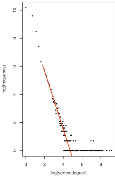
Again we make use of the pedigree graph represen-tation where inbred lines are represented as vertices and each single-cross hybrid is represented as an edge between two vertices as shown in Figure 2. In this graph, the degree of a vertex (i.e., the number of edges incident to the vertex) therefore equals the number of distinct single-cross hybrids of which the inbred line is a parent. Figure 4 shows the empirical distribution of these degrees on a log scale for the entire RAGT grain maize breeding pool. The observed long-tailed behavior of the empirical distribution is not unexpected as most inbred lines only have a limited number of children, while inbred lines with higher progeny numbers (i.e., the tester lines) are rare. In an attempt to parametrize the underlying distribution from which the observed vertex degrees were drawn, several candidate distribu-tions among which the Poisson, geometric, discrete log-normal, and discrete power-law distributions were fitted by means of likelihood maximization. The best fit was observed for the discrete power-law distribution with a left threshold value of 6 that is indicated as a straight line on Figure 4. The fit of this distribution is, however, insufficient as indicated by the significantly large Kolmogorov–Smirnov D-statistic, where significance is determined by means of the parametric bootstrap procedure described by Clausetet al. (2009).
As no conclusive evidence on the underlying distri-bution of the observed vertex degrees was found, we
prefer to sample inbred lines from the full RAGT graph directly. However, taking a representive sample from a large graph is not a trivial task. The sample quality of various published graph sampling algorithms seems to be highly dependent on the properties of the graph.
TABLE 2
Description of each step that is performed during a single iteration of the simulation routine
Step Description
1 Sample 400 vertices from the pedigree graph by means of the ‘forest fire’ algorithm: Indirect sampling of hybrids
Indirect sampling of multi-environment trials
2 Partition sampled inbred lines incheterotic groups by means of the Dsatur vertex coloring algorithm 3 Simulate 8 breeding cycles on each of thecheterotic groups
4 Simulate phenotypic records on the sampled hybrids
5 Reduce the number of sampled hybrids by gradually increasing CDmin
6 Reduce the number of genotyped inbred lines by means of the greedy densestk-subgraph algorithm
7 SelectqSSR markers with maximal genome coverage
8 Determine the prediction accuracy ofe-SVR and BLP using the reduced set of training examples
The goal is to find the optimal trade-off between the number of genotyped inbred lines and the size of their molecular fin-gerprint, when the total genotyping budget is fixed.
To decide which sampling routine is optimal for the RAGT data, we first need to decide on a measure of sample quality. We compare the empirical cumulative distribution (ECD) of the vertex degrees in the full graph with those ECDs of 100 samples containing 400 vertices. From these ECDs, we calculate the average Kolmogorov–Smirnov D-statistic for each examined sampling routine. For the RAGT data, the ‘‘forest fire’’ vertex sampling approach resulted in the smallest averageD-statistic compared to the alternative methods described by Lescovec and Faloutsos (2006). This
sampling routine starts by selecting a vertex v0 uni-formly at random from the graph. Vertexv0now spreads ‘‘the fire’’ to a random selection of its neighbors, which are then in turn allowed to infect a random selection of their own neighbors. This process is continued until exactly 400 vertices are selected. If the fire dies out before the sample is complete, a new starting vertex is selected uniformly at random. The number of neigh-bors that is infected at each selected vertex is obtained as a random draw from a geometric distribution where the parameterpwas set to 0.62, as this value resulted in the best average sample quality. All hybrids for which both parents were sampled (i.e., the edges of the subgraph) have associated phenotypic records and as such indirectly sample a set of multi-environment trials (METs). All hybrids that were not indirectly selected by the inbred line sample, but do have phenotypic records in the sample of METs, are included in the selection as data connecting check varieties. Despite the fact that the RAGT data already provide phenotypic records for the selected hybrids and check varieties, we replace these by simulated measurements as we want to be able to assess the actual prediction accuracy ofe-SVR and BLP under various levels of data quality.
The simulation of these phenotypic records for the sampled hybrids starts by partitioning the selected inbred lines into heterotic groups. This partitioning should ensure that the two parents of each single-cross hybrid always belong to distinct heterotic groups, while the total number of groups needs to be minimized. The graph theory equivalent of this problem is called the ‘‘vertex coloring problem,’’ which, as all previously described graph theory problems, belongs to the com-plexity class of NP-hard problems. The minimum number of colors (i.e.,heterotic groups) is called the chromatic number of the graph. The vertex coloring problem has been extensively studied in graph theory literature ( Jensenand Toft1995) and several efficient
heuristics are available. The greedy desaturation algo-rithm or Dsatur published by Bre´ laz (1979) is often
used as a benchmark method to assess the efficiency and precision of newly developed vertex coloring algo-rithms. Its good performance on a variety of graphs and easy implementation makes it the method of choice for designating inbred lines to heterotic groups at each iteration of the simulation routine.
Once the chromatic numberchas been determined for the sampled set of inbred lines, an entire breeding program is simulated starting from c open-pollinated varieties and resulting incunrelated heterotic groups. The simulation of this breeding program mimics the maize breeding program of the university of Hohenheim as described by Stich et al. (2007) and modified by
Maenhout et al. (2009). In short, the simulation
routine uses the proprietary linkage map of the breed-ing company RAGT R2n containbreed-ing 101 microsatellites and adds an additional 303 evenly distributed, simu-lated SSRs. It also generates 250 QTL loci of the selection trait (e.g., yield), which are randomly posi-tioned on the genetic map. The number of alleles for each SSR or QTL is drawn from a Poisson distribu-tion with an expected value of 7. Each simuladistribu-tion starts by generating an initial base population in Hardy– Weinberg equilibrium. Allele frequencies for each locus are drawn from a Dirichlet distribution and used to calculate the allele frequencies in each of the c sub-populations assuming anFstvalue of 0.14. We perform 8 breeding cycles where each cycle consists of 6 gener-ations of inbreeding and subsequent phenotypic selec-tion based on line per se or testcross performance as described by Stichet al. (2007). The result is a set of 400
highly selected inbred lines partitioned in cunrelated heterotic groups. Within each of these groups, the simulated inbred lines are randomly assigned to the sampled inbred lines and a genotypic value is generated for each interheterotic hybrid by summing the effects of the 250 QTL alleles of both parents and adding a normally distributed SCA value. The size of the SCA variance component depends on the heritability of the trait under consideration, but is assumed to be only1 8 of the total nonadditive variance (SCA 1 G 3 E and residual error) as this was the average of observed ratios for the traits grain yield, grain moisture contents, and days until flowering in the actual RAGT data. The genotypic values of the check varieties are generated from a single normal distribution where the variance is the sum of the additive variance and SCA variance of the sampled hybrids. The simulated genotypic values of hybrids and check varieties are used to generate phenotypic records according to the sampled MET data structure, assuming a single replication in each location of a MET. This implies thatG3Eeffects are confounded with the residual error and only a single effect is drawn from a normal distribution where the variance is7
8 of the total nonadditive variance. The main environmental effect of each location is also drawn from a normal distribution for which the variance is twice the additive variance of the hybrids.
as this approach should result in ane-SVR model with a superior prediction accuracy (Maenhoutet al. 2010).
To avoid selections of closely related hybrids, the variance–covariance matrix of the genotypic effects is fitted as a scaled identity matrix. The resulting PEV matrix of the random genotypic effects is used to iteratively select a smaller subset of the sampled hybrids by gradually increasing the minimum required pre-cision of each pairwise contrast in the selection. Initially, the required CDminvalue is set to 0, which implies that all hybrids are selected. The next examined level of precision requires CDmin.0, which effectively excludes selections containing disconnected individuals. More stringent levels of precision are enforced by requiring CDmin.qp, whereqpis thepth quantile of the observed distribution of CD values in the complete sample andp ranges from 0 to 0.875 in steps of 0.125. Defining CDmin values as quantiles allows us to compare the obtained prediction accuracies over the different samples of the simulation routine.
For each level of CDmin, the number of genotyped inbred lines is reduced from 400 to 50 in steps of 50, while at the same time the number of markers in the molecular marker fingerprint is increased from 50 to 404. For each combination of CDminand number of genotyped inbred lines, the BLUPs of the selected hybrids are used to construct ane-SVR and a BLP-based prediction model. In fact, the prediction accuracy of both methods is verified by randomly assigning the BLUPs to one of five groups. For each of these groups, a separate e-SVR and BLP prediction model is constructed using all BLUPs in the remaining four groups as training data. The resulting prediction model is then used to make predictions on the hybrids in the selected group (i.e., the validation data). Combining the predictions of all five models allows us to obtain a measure of prediction accuracy by correlating them against the simulated genotypic values.
Simulation results:We expect that enforcing a mini-mum required pairwise contrast precision CDmin . 0 results in a selection of BLUPs that has greater accuracy compared to the full set of hybrids. In Figure 5 this BLUP accuracy is plotted against CDmin and the maximum number of inbred lines for each of the three examined heritability levels. Each point on these wire-frame surfaces represents the squared Pearson correla-tion between the BLUPs and the actual, simulated genotypic values of the selected hybrids at that partic-ular level of CDminand number of parental inbred lines, averaged over 100 iterations of the simulation routine. We can see that an increase in CDminresults in an almost linear increase in BLUP precision for each heritability level. This effect is especially pronounced for the lowest heritability level h2 ¼ 0.25. As expected, the BLUP
precision is not influenced by the number of parental inbred lines.
Figure 6 presents the prediction accuracy of both e-SVR and BLP for increasing values of the minimum
required contrast precision CDmin and a decreasing number of genotyped inbred lines. The height of each point in the wireframes represents the average pre-diction accuracy, expressed as a squared Pearson corre-lation, over 100 iterations of the simulation routine. For each of the examined heritability levels,e-SVR generally performs better than BLP. The negative effect of disconnected hybrids in the selection of training exam-ples is visualized as the sharp increase in prediction accuracy when the minimum required contrast preci-sion is slightly constrained from CDmin¼0 to CDmin.0 . This effect is more pronounced for BLP than fore-SVR. Increasing CDmin any further generally decreases the prediction accuracy, especially for traits with lower heritability. This observation implies that, at least for the RAGT data set, a larger number of training examples of lower data quality is to be preferred over a smaller selection of hybrids for which more and better connected phenotypic information is available, as long as disconnected individuals are excluded.
BLP ande-SVR do not take a unanimous stand on the optimal number of genotyped inbred lines. For BLP, the optimum seems to lie somewhere around 100 inbred lines forh2¼0.25 and 150 forh2¼0.50 andh2¼0.75, the
equivalent of fingerprint sizes of 202 and 134 SSR Figure5.—Accuracy of the genotypic value BLUPs of the hybrids selected using the described graph-based procedures. The three examined heritability levelsh2¼0.25,h2¼0.5, and h2 ¼ 0.75 are represented by the bottom, middle, and top
markers, respectively. This optimum is, however, less pronounced for the higher heritability levels. Fore-SVR, the optimal number of inbred lines is 150, 200, and 350 forh2¼0.25,h2¼0.5, andh2¼0.75, respectively. At the
highest heritability level,e-SVR seems to prefer training sets of maximum size, at the cost of a very small molecular marker fingerprint size. The observed behav-ior of both BLP ande-SVR is consistent with the results of a previous study (Maenhoutet al. 2010) where it was
shown that BLP is less sensitive to a reduction of the number of training examples compared to e-SVR, as long as the molecular marker fingerprint is dense.e-SVR on the other hand, although requiring a training set of
considerable size, handles smaller or less informative molecular marker fingerprints better than BLP.
DISCUSSION
This article presents three selection problems that are relevant to the budget-constrained construction of a genomic prediction model from available genetic eval-uation data. The first problem considers the selection of exactlypindividuals from a set oftcandidates that will be genotyped to serve as training examples for the construction of the prediction model. This selection should be optimal in the sense that a linear mixed Figure 6.—Average prediction accuracy of
model analysis of the associated phenotypic records should result in a set ofpBLUPs of genotypic values that have the highest precision of all possible selections. By defining the precision of a selection as the minimum generalized coefficient of determination of a pairwise contrast, this selection problem can be translated to the discretep-dispersion problem from the field of graph theory. The reduction of this problem to a set of maximum clique problems allows us to visualize the trade-off between selection size and selection quality. The greedy nature of a breeding program does un-fortunately bias the presented selection approach to-ward high-performing individuals. These are generally tested more thoroughly than their low-performing colleagues. As the latter generally have only a few associated phenotypic records, the pairwise contrasts involving these individuals have a low precision, which in turn makes their selection by the described pro-cedure very unlikely. As a consequence, the resulting genomic prediction model is likely to overestimate the capabilities of the low-performing individuals. To avoid this bias, the selection procedure should optimize two objectives simultaneously: (1) maximizing the mini-mum precision of all pairwise contrasts in the selection and (2) maximizing the genetic variance in the selec-tion. Even if one would succeed in finding an acceptable trade-off between these conflicting objectives, the esti-mates of the genotypic value of low-performing individ-uals will always suffer from large standard errors, which makes them unreliable training examples.
The second problem we discuss deals with the selection of exactlyqmolecular markers from a set oft candidates for which the relative positions on a genetic map are known. To guarantee that the selection has an optimal genome coverage, we maximize the minimum intermarker distance. We show that this problem can be translated to a one-dimensional discrete p-dispersion problem for which an exact algorithm is available.
The third problem is specific to hybrid breeding programs and entails the selection of exactlykparental inbred lines such that the number of single-cross hybrids in the selection is maximized. If we represent the inbred lines as vertices of a graph and each single-cross hybrid as an edge between its parental vertices, this problem can be translated to the densest k-subgraph problem, which we solve by using a greedy heuristic.
The presented solutions to the three selection prob-lems are put into practice in a simulation study in which the goal is to find the optimal number of training examples for the construction of e-SVR and BLP pre-diction models with maximal prepre-diction accuracy under a fixed genotyping budget. At each iteration of the simulation routine, inbred lines, hybrids, and their associated phenotypic data structure are sampled from actual genetic evaluation data. The number of training examples is gradually reduced by putting constraints on the data quality and the number of genotyped inbred
lines. The results indicate that selections of training examples containing disconnected individuals are det-rimental to the prediction accuracy of bothe-SVR and BLP. More stringent data quality constraints are, how-ever, not necessary.e-SVR performs best if the number of parental inbred lines (i.e., the number of training examples) is maximized at the cost of a reduced genome coverage. BLP on the other hand performs best when trained on a smaller set of training examples for which a dense fingerprint is available.
Despite the fact that these conclusions are most likely specific to maize breeding programs and possibly even specific to the heterotic groups and breeding methods used by the data-providing breeding company, the presented graph-based data selection algorithms should prove themselves to be useful for the construction of genomic prediction models in other plant and animal species as well. Evidently, more species-specific case studies are required to ascertain this claim.
The authors thank the people from RAGT R2n for their unreserved and open-minded scientific contribution to this research.
LITERATURE CITED
Asahiro, Y., K. Iwama, H. Tamakiand T. Tokuyama, 2000 Greedily
finding a dense subgraph. Algorithmica34:203–221.
Battiti, R., and M. Protasi, 2001 Reactive local search for the
max-imum clique problem. Algorithmica29:610–637.
Bernardo, R., 1994 Prediction of maize single-cross performance
using RFLPs and information from related hybrids. Crop Sci.
34:20–25.
Bernardo, R., 1995 Genetic models for predicting maize single-cross
performance in unbalanced yield trial data. Crop Sci.35:141–147. Bernardo, R., 1996 Best linear unbiased prediction of the
perfor-mance of crosses between untested maize inbreds. Crop Sci.
36:50–56.
Bernardo, R., 2008 Molecular markers and selection for complex
traits in plants: learning from the last 20 years. Crop Sci.48:
1649–1664.
Bomze, M., M. Budinich, P. Pardalosand M. Pelillo, 1999 The
maximum clique problem, pp. 1–74 inHandbook of Combinatorial Optimization, Supplement Vol. A, edited by D.-Z. Duand P. M.
Pardalos. Kluwer Academic, Dordrecht, The Netherlands.
Bre´ laz, D., 1979 New methods to color the vertices of a graph.
Commun. Assoc. Comput. Mach.22:251–256.
BuenoFilho, S., and S. G. Gilmour, 2003 Planning incomplete
block experiments when treatments are genetically related. Bio-metrics59:375–381.
Carraghan, R., and P. M. Pardalos, 1990 An exact algorithm for
the maximum clique problem. Oper. Res. Lett.9:375–382. Chakrabarti, M. C., 1964 On the C-matrix in design of
experi-ments. J. Indian. Statist. Assoc.1:8–23.
Clauset, A., C. R. Shaliziand M. E. J. Newman, 2009 Power-law
distributions in empirical data. SIAM Rev.51:661–703. DeMeyer, H., H. Naessensand B. DeBaets, 2004 Algorithms for
computing the min-transitive closure and associated partition tree of a symmetric fuzzy relation. Eur. J. Oper. Res.155:226–238. Erkut, E., 1990 The discretep-dispersion problem. Eur. J. Oper.
Res.46:48–60.
Erkut, E., Y. Ulkusaland O. Yenicerioglu, 1994 A comparison of
p-dispersion heuristics. Comput. Oper. Res.21:1103–1113. Feige, U. and M. Seltser, 1997 On the densestk-subgraph
prob-lem. Technical Report CS97-16, Weizmann Institute, Rehovot, Israel.
Foulley, J., J. Bouix, B. Goffinet and J. M. Elsen, 1990
Statistical Methods for Genetic Improvement of Livestock, edited by D. Gianolaand K. Hammond, Springer-Verlag, Heidelberg.
Gianola, D., and J. B. C. H. M.vanKaam, 2008 Reproducing kernel
Hilbert spaces regression methods for genomic assisted predic-tion of quantitative traits. Genetics178:2289–2303.
Hayes, B. J., P. J. Bowman, A. J. Chamberlainand M. E. Goddard,
2009 Genomic selection in dairy cattle: progress and chal-lenges. J. Dairy Sci.92:433–443.
Heiligers, B., 1991 A note on connectedness of block designs.
Metrika38:377–381.
Henderson, C. R., 1975 Best linear unbiased estimation and
predic-tion under a selecpredic-tion model. Biometrics31:423–447. Henderson, C. R., 1984 Applications of Linear Models in Animal
Breed-ing.University of Guelph Press, Guelph, Ontario, Canada. Jensen, T., and B. Toft, 1995 Graph Coloring Problems.Wiley, New York.
Kennedy, B., and D. Trus, 1993 Considerations on genetic
connect-edness between management units under an animal model. J. Anim. Sci.71:2341–2352.
Laloe´, D., 1993 Precision and information in linear models of
ge-netic evaluation. Genet. Sel. Evol.25:557–576.
Laloe´, D., F. Phocasand F. Me´ nissier, 1996 Considerations about
measures of precision and connection in mixed linear models of genetic evaluation. Genet. Sel. Evol.28:359–378.
Lescovec, J., and C. Faloutsos, 2006 Sampling from large graphs,
pp. 631–636 inProceedings of the 12th ACM SIGKDD International Conference on Knowledge Discovery and Data Mining, Association of Computing Machinery, New York.
Maenhout, S., B. DeBaets, G. Haesaertand E. VanBockstaele,
2007 Support vector machine regression for the prediction of maize hybrid performance. Theor. Appl. Genet.115:1003–1013. Maenhout, S., B. DeBaets, G. Haesaertand E. VanBockstaele,
2008 Marker-based screening of maize inbred lines using sup-port vector machine regression. Euphytica161:123–131. Maenhout, S., B. DeBaetsand G. Haesaert, 2009 Marker-based
estimation of the coefficient of coancestry in hybrid breeding programmes. Theor. Appl. Genet.118:1181–1192.
Maenhout, S., B. DeBaetsand G. Haesaert, 2010 Prediction of
maize single-cross hybrid performance: support vector machine regression versus best linear prediction. Theor. Appl. Genet.120:
415–427.
Meuwissen, T. H. E., B. J. Hayes and M. E. Goddard,
2001 Prediction of total genetic value using genome-wide dense marker maps. Genetics157:1819–1829.
Naessens, H., H. DeMeyerand B. DeBaets, 2002 Algorithms for
the computation of T-transitive closures. IEEE Trans. Fuzzy Syst.
10:541–551.
O¨ sterga˚ rd, P. R. J., 2002 A fast algorithm for the maximum clique
problem. Discrete Appl. Math.120:197–207.
Patterson, H. D., and R. Thompson, 1971 Recovery of
inter-block information when inter-block sizes are equal. Biometrika58:
545–554.
Ravi, S., D. Rosenkrantz and G. Tayi, 1991 Facility dispersion
problems: heuristics and special cases. Lecture Notes Comput. Sci.519:355–366.
Stich, B., A. E. Melchinger, H. P. Piepho, S. Hamrit, W. S chip-prack et al., 2007 Potential causes of linkage disequilibrium
in a european maize breeding program investigated with com-puter simulations. Theor. Appl. Genet.115:529–536.
Tomita, E., and T. Seki, 2003 An efficient branch-and-bound
algo-rithm for finding a maximum clique. DIMACS Ser. Discrete Math. Theoret. Comput. Sci.2731:278–289.
Warshall, S., 1962 A theorem on Boolean matrices. J. Assoc.
Com-put. Mach.9:11–12.
Yu, J., G. Pressoir, W. H. Briggs, I. VrohBi, M. Yamasakiet al.,
2006 A unified mixed-model method for association mapping that accounts for multiple levels of relatedness. Nat. Genet.38:
203–208.
Communicating editor: I. Hoeschele
APPENDIX: IDENTIFYING DISCONNECTED PAIRS OF INDIVIDUALS
Appendix A: By examination of the PEV matrix
If we analyze the available genetic evaluation data with a linear mixed model according to Equqation 1, where the variance structure is simplified to
Var u e ¼
Is2g 0 0 Is2e
;
we can express the prediction error variance matrix as (Henderson1984)
PEVðˆuÞ ¼ ðZ9MZ1IlÞ1s2 e; wherel¼s2
e=s2gandMis the orthogonal projector on the column space of matrixXasM¼IXðX9XÞ 1
X9. The matrix productZ9MZis in fact the information matrix of the genotypic effects if we would consider both environments and genotypic effects as fixed and analyze the data as a block design in a linear least-squares setting. Chakrabarti
(1964) proves that if such a block design is fully connected (i.e., all elementary contrasts are estimable in a least-squares sense), the rank of this information matrix equalst1, wheretis the number of fitted genotypic effects. Furthermore, Heiligers(1991) proves that in case the information matrix has a lower rankt p, where p$ 2, the design is
Appendix B: By computing the transitive closure
If VarðuÞis not a diagonal matrix, the block diagonal structure ofZ9MZis not preserved in the PEV matrix. One could of course examine the structure ofZ9MZinstead, but this matrix is generally not available. It might therefore be easier to identify disconnected pairs of individuals by determining the transitive closure of their adjacency matrix. This is a symmetric, Booleant3tmatrix where the element on rowiand columnjis set to 1 if individualsiandjhave been evaluated in a common environment and 0 otherwise. For the example in Figure 1, this adjacency matrix looks like
A¼
1 1 0 0
1 1 0 0
0 0 1 1
0 0 1 1
2 6 6 4
3 7 7 5:
The transitive closure of this matrix is again a symmetric, block-diagonalizable, Boolean matrix that can be interpreted in a similar way asZ9MZWarshall(1962) describes a concise and efficient algorithm for computing the
transitive closure of an adjacency matrix that has a worst-case complexity ofO(t3). More advanced algorithms are