Performance evaluation of a bufferless NxN synchronous Clos ATM switch with priorities and space preemption

Performance Evaluation of a

Bufferless

N

x

N

Synchronous Clos

ATM

Switch with Priorities

and

Space Preemption

Arne

A.

Nilsson

Fuyung

Lai

Harry

G. Perros

Center for Communications and Signal Processing

Department Electrical and Computer Engineering

North Carolina State University

TR-90j17

Performance Evaluation of a Bufferless

NxN

Synchronous Clos ATM Switch with Priorities and

Space Preemption

*

Arne A. Nilsson and Fuyung Lai

Department of Electrical and Computer Engineering

Center for Communications and Signal Processing

North Carolina State University

Raleigh, N.C. 27695-7914

Harry G. Perros

Department of Computer Science

Center for Communications and Signal Processing

North Carolina State University

Raleigh, N.C. 27695-8206

Abstract

We consider a synchronized bufferless Clos ATM switch with input cell processor queues. The arrival process to each input port of the switch is assumed to be bursty and it is modeled by an Interrupted Bernoulli Process. Two classes of cells are considered. Service in an input cell processor queue is head-of-the-line without preemption. In addition, space preemption is used. That is, a high priority cell arriving at afull queue takes the space occupied by the low priority cell with the least waiting time in the queue but not the one in service. Each cell processor queue is modeled as a priority IBP/Geo/l/K+l queue with space preemption. We present an exact analysis of the priority queue. The results obtained are then used in an approximation algorithm for the analysis of the ATM switch.

1

Introduction

Broadband ISDN is a promising communications infrastructure for the future. BISDN is conceived as an all-purpose digital network. It will provide an integrated access that will support a wide variety of applications for the customers. The Asynchronous Transfer Mode (ATM) has been strongly promoted as the target transfer mode solution for broadband ISDN. ATM is a high-bandwidth, low-delay, packet-like switching and multiplexing technique. ATM is capable of efficiently multiplexing a number of highly bursty sources, such as voice, file transfer, and video.

In recent years, several types of ATM switch architectures have been proposed. One important class of architectures is based on multi-stage interconnection networks. There are buffered or unbuffered switching elements in a multi-stage interconnection network. In the unbuffered case, there may be buffers at the input ports or at the output ports of the switch. This type of structures have been reported in Turner [1], Narasimha

[2],

Huang and Knauer [3], Giacopelli, Littlewood, Sincoskie

[4],

and Tobagi and Kwok [5]. Some switch architectures provide full connectivity between the input and output ports, such as the bus-matrix switching architecture (Nojima et al

[6]),

the knockout switch (Yeh, Hluchyj, and Acampora [7]), and the integrated switch fabric (Ahmadi et al

[8]).

Other architectures that have been proposed are the shared memory and the shared medium architectures. In the shared memory architecture, a single memory is shared by all input and output ports. There is a single controller to process the incoming and outgoing cells which are stored in the same memory. The examples of this type of architecture are shown in Devault, Cochennec, and Servel [9], and Kuwahara, Endo, and Ogino

[10].

In the shared medium type of architectures, arriving cells are multiplexed onto a parallel bus. An example of this architecture is in Suzuki et al [11]. A good review of ATM switch architectures is given in Tobagi [12]. Some approximate analysis of the ATM switches have been shown in Karol, Hluchyj and Morgan [13], Hluchyj and Karol

[14],

Patel

[15],

Yoon, Lee, and Liu [16], Shaikh, Schwartz, and Szymanski [17], Oie, Suda, Masayuki, and Miyahara [18].

to a threshold. After that only high priority cells are admitted. The partial buffer sharing scheme is easier to implement, though it has a lower performance than the space priority scheme presented above (see Korner

[21]).

For a litterature review of ATM related papers see Perros

[22].

In this paper, we consider a. bufferless ATM switch with finite buffers at the input ports. The switch fabric is a Clos three-stage interconnection network. The arrival process to each input port of the switch is assumed to be bursty (see Heffes, and Lucantoni

[23])

and is modelled by an Interrupted Bernoulli Process. Each input cell processor queue is modelled as a two-class priority queue with head-of-the-line service priority and with no preemption. In addition, space preemption is assumed. An approximate analysis of this switch has been reported ill Nilsson, Lai, and Perros [24] without priorities and space preemption. We now proceed to describe the switch under study in detail.

2

Model description

Let us consider an N x N Clos cell switch, as shown in Figure 1. There are three stages in the switch. At each stage, there are n or

VN

number of bufferless switching elements. Each switching element is an n x n crossbar switch.For each input port, there is a finite queue served by a cell processor. In this model, we analyze the cell processor queue as a two priority head-of-the-line system. There are two classes of cells, high and low priority. If an arriving high priority cell finds the buffer of the cell processor full, it will throw out a low priority cell with the least waiting time in the system, but not the one in service. An arriving low priority cell is lost if it finds the buffer full. An arriving high priority cell is lost only if the buffer is full with high priority cells. We refer to this priority scheme for buffer occupancy as space preemption. The cell processor is responsible for determining the output port of a cell and then transmitting the cell through the switch fabric. The operation of the Clos switch is synchronous. That means, at the beginning of a time slot all the busy cell processors will launch a cell through the switch. A cell will successfully get through the switch if it finds a free path to the sought output port.No contention takes place at the 1st stage of the Clos ATM switch. The cells in the switch will compete for the output lines at the 2nd and the 3rd stages.

In

a switching element, if more than one input line compete for the same output line, one of the input lines will get through. This input line is randomly selected. If a cell is blocked in the switch, it is assumed that the switching element will notify the cell processor. The transmission of a cell will be aborted. The cell processor will retransmit the cell at the beginning of the next time slot. The retransmissions will continue until the cell is successfully transmitted through the switch.

1

...m-

₁

2 0

0 2

0 1 0

--m-

••

n n

n+l

0l

n+l

0

•

0

2n 2n

0 ₀

0

•

0 ₀

• 0

• •

• •

N-n+l ....[IID-_• 0 0

.

N-n+l

• • n • 0 n 0

0 •

....[IID- • 0 • 0

N N

the switch. A cell that arrives at an idle cell processor in the middle of a slot of the ATM switch is not transmitted until the beginning of the next time slot of the ATM switch.

The arrival process to each input port of the ATM switch is modeled as a discrete time Interrupted Bernoulli Process(IBP), see Figure 2. It can be shown (see Nilsson, Lai,

1-p

p

1-q

Figure 2: The Markov chain of the IBP process.

q

and Perros [24]) that the mean interarrival time E(i) is equal to

E{l}

=

(2 -

p - q)

a(l - q)

the squared coefficient of variation of the interarrival time, C2

, is obtained as

(1)

(2)

02

==

1

+

a

((1 -

p)(3 -

q) _

2)

+

0.2

(1 -

q)2

.

(2 -

p - q)2

(2 _

p _ q)2

It can also be shown that the probability for a cell successfully passing through the Clos ATM switch ,1 - a , is

1- a = Average number of busy output lines at the 3rd stage

Average number of busy input lines at the 1st stage N

~ [3]

LJPi

i=l N

LPi

i=l

(3)

where p!3) is the ith output line utilizations of the switching elements in the 3rd stage of the

3

Exact analysis of the IBP /Geo/l • queue with finite

capacity, head-of-the-line priority and space

pre-emption:

Let us consider a cell processor queue. It is obvious from the previous section that the total time it takes for the cell processor to transmit successfully a cell through the switch fabric is geometrically distributed with probability a . Therefore, a cell processor queue can be modeled as a discrete IBP /Geo/l with finite buffer, HOL priority, and space preemption, as shown in Figure 3. In the analysis of this queueing system we consider the successive arrival

K

~

IBP

Figure 3: The finite buffer queueing system with priorities and space preemption scheme.

points as shown in Figure 4. These arrival points are the imbedded Markov points of the queueing system. Our approach is to focus attention on arrival instants and the number of

high and low priority customers seen by an arriving customer.

(m,n)

S·

...

..

L

J

~I

I slots

(i,j)

I

f

I

~

Figure 4: The evolution of the number of customers in the system.

3.1

Queue Length Distribution

andj is the number of low priority cells in the queue. To analyze the system, we need the following notation :

{3 : the probability that an arriving cell is a high priority cell.

Pi,i : the probability that an arriving cell finds i high priority and j low priority cells in the queue with a busy server.

Po

the probability that an arriving cell finds an empty system.

i :

the interarrival time of the cell.

X : the number of slots needed for a cell to be successfully transmitted to the output line.

We define

and

P[i

==

l]

1~ 1

P[x

==

l]

==

(1 - U)Ui- 1, i

2:

1,

where a, is the probability of an interarrival time of 1slots, and o is the probability of a cell to be blocked in the Clos ATM switch and retransmitted. From Nilsson, Lai, Perros [24], we have

"i'

the steady state probability that an arriving cell finds j customers in the system immediately prior to its arrival. This is the steady state probability in a single class of IBP

IGEO II

queue with finite buffer. Thus, we have

Po

,0

Po,o

,1

Let us define

bo

==

A(u),

where A(z) is the z-transform of the probability distribution of the interarrival time. In order to obtain P..._1.,3 we need to study the system at instants of arrivals. In steady state, we

have

~.

.

{3K~-j

P. .

~

(

~

) u

'-(n-i+l)(l _ u)(n-i+l)a,

1.,3 L..J n,3L..J n - 1,

+

1

n=i-l 1=1

L

OO

( I ) l-(K-i-i)(l _ )(K-i-i) +t:lPK-1-ji+1_,.." K · ·_{- ) - 1 ,} a U

a,

K-1-(;-1) 00 ( l )

+(1 -

fJ) ~i Prn,;-l

f;

m _ i _{U'-(rn-i)(l - U)(rn-i)a,}

(3(Pi-l,jbO

+

Pi,jb1

+ ... +

PK-1-;,jbK- i- j)

+

{3PK -1-i,j+lbK-i-j

+(1 -

(J)(P

i,j - l bO

+

Pi+1,i-l bl

+ ... +

PK-i,i-lbK-i-i)

for i,j >

°

and i

+

j < K,

and

K-1 00 ( l )

Pi,o

=

fJn~l Pn,o

f;

n _ i

+

1 u

'- (n - i + l ) ( l - u)(n-i+l)a,

+fJ(PK,o

+

PK-1,d

f (

K ':i ) u

'-(K-i)(1 - u)(K-i)a,

1=1

{3(Pi - 1,obo

+

Pi,ob1

+ ...

+

PK-l,obK -i )

+{3PK,obK-i

+

(3PK - 1,l bK -i

for K

>

i

>

0, and j

==

0, and

K-l-(j-l) 00 ( 1 )

Po,; (1 - fJ)

?;

~

Pn,;-l n _u'-n(l - Ural

K-1K-1-n 00 ( 1 )

+

~ ~

""'

~ u

' (m + l + n

-j_{)( l _ u)(m+l+n-}j_)az

L...J. L...J L...J m,n m

+

1

+

n _ j

n=3 m=O 1=1

+fJ

t

PK-n,nf ( K '. · ) u'-(K-i)(l_ u)(K-;)a,

n=i+l 1=1 J

+(1 -

fJ)

t.

PK-n,n

f (

K

~

. ) u'-(K-;)(l - u)(K-i)a,

n=3 1=1 J

(1 -

(3)(PO,i-l bO

+

P1,i-l b1

+ ...

+

PK -i ,i - lbK - i )

+PO,i bl

+

P1,i b2

+ ...

+

PK-l-i,jbK-j)

+

(1 -

(J)PK-i,jb K-;

+PO,j+l b2

+

P1,;+lb3

+ ...

+

PK -1-(;+I),;+1 bK-;)

+

PK-(;+l),;+lbK - ;

+ ...

+PO,K-1bK-i

+

P 1,K-lbK-i

+Po,KbK- i

for i

==

0, and K

>

j

>

0,

For the case i

+

j

==

K,

we have

00 00 00

PK,O

=

PK,O

L

u'a,

+

fJPK-1,o

L

u'a,

+

fJPK-1,1

L

u'a,

and

00 ex>

PO,K (1-(3)PO,K

L

u'a,

+

(1-(3)PO,K-1

L

u'a,

1=1 1=1

and

00 00

{3Pi-1,K- i

L

u'a,

+

{3Pi-1,K-i+1

L

u'a,

+

1=1 1=1

00 00

(1 - (3)Pi,K-i

L

u'a,

+

(1 - (3)Pi,K-i-1

L

u'a,

1=1 '=1

for K

>

i

>

o.

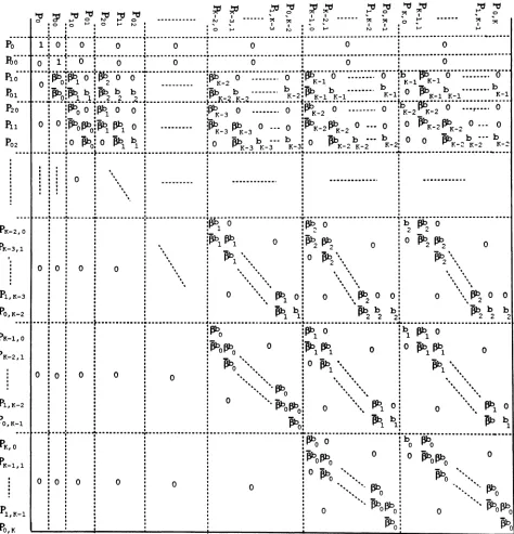
From the above equations, we obtain the transition probability matrix of the system shown in Figure 5. Thus, the steady state probability, Pi,j, can be computed using a numerical

o o o , ,_,

_.

,

.

,

..

, o o ~0f3b0 0

0 _~O ,,,_,

0

.

,,,_{, pho}

.._.. ~0f3b0 0 ~O o o o o ,

_.

, ,

...

o o o o o o o o o o o o

;r; ~ ::a~ ~~ ;J:'~ ~~~ :JJ~

~~~~~~~ 1 : ; J f " " 0 I I 0 ~I : . 0

o •0 '6

e.

~ ~ ~: .!" ~ ~ ~ •~ !" ~ ~ .~ ~ .. ~

: : : ' :0 ~ w "':O~ ",...,:..., ...,

• - - .1 • • • •~. • • _~• • • • • • • __ • • • •~• • • _ • • • __ • _ • • • _ . . . __ • _ • • • • _ • • • _ • • • • • _ • • _ • • • • • • • __ • • _ • • • • __ • _ • • _ • • • • __ • • _ • __ • _ • __ • • • • • • _ • _ • • • • •'• • • • • •

1 : 0 : 0 : 0 : 0 : 0 : 0 : 0

oooo • .:.oooo.

i

J

oo • • • • oo.oo • •~• • • • • • • • oo• • • • • • • •t ~ oo• • • • • • • • • • • • • • • • : • • • • • • • • • • • • • • • • • • • • • • • • • • • • • •

0 : 1 : 0 : 0 : 0 : 0 : 0 : 0

....:

~+~

..;;

+~

..

0"

·o··f··· ···

i~····

0""'::::::::'

C)··

+Ilfr'"

0'"'::::::.~''r;"

1J:i·..

13£!..••

'0"'::::::::'0"

0: 0: 1 : 2 : : K-2 : K-l : x-i K-l

: An :An b : An b b • :iih b ... b :iin b ... --. b : 0 Olo.. b ... -- ... b

: t"""o:.'·i l : t"""2 2 , , : ...1(_" _ K-2. t"""K-l x-i K-I, P"'"'K-I K-I K-I

.oooo - • • • • • • • • • • •'t • • • • • • • • • •h."...···t·.,~·.. ·K.~••••••••••••••i···t···~···..··

: :f3b

o 0 :~l 0 0 : :~K-3 0 0 :~K-2 0 0 :bK _ 2 K-2 0 1' 0

.

.

"

.

.

o : 0 :~O~O~~l ph1 0 : ~ Pi? 0 ... 0 ~~K-2f3k?K 2 0 ... 0 ~ 0 ~K-2pbK-2 0 .... 0

: : . : • K-3 K-3 • - • _

• I Ah : An b " - b b ' 'Bh b · · · b • 0 0 Ah b··· b

: : 0 t"""o: 0 ""-1 1: :0 f3b_{K - 3} K-;-- K-3: 0 P""'K-2 K-2 K-2: "-K-~ K-2 K-~

....: ~...•...~ ~ ~ -:-

_

.

: : : : : : :

n :

: , : :

:

:

• - 0 : , I : • • • • • • • • • • • • • : • • • • • • • • • • • • • • :

: : • ' . : I • ,

: : : ' , : : : :

: : : : : : :

: : : : : : :

. . ' I ' , I

~ .:. •••••••••••••••••••••••••••••·~~1··0···

t

~··o···~·b··~··o··· .

• • 2 2 2

$hl phl 0 .~ ~ 0 0 ~ ~

~l

0

~.>\

~2.>\\

' " .., "', "" '" 9,

" , phI 0 0 \\ ~ 0 0 0 \ \~ 0 0

b 'an b b An b b

phI I, """"2 2 2, "-2 2 2

.... ····r···.··· ...•...~ .

'Ah '

:t"""0 :1J:>1 0 b₁ phI 0

'~0f3b0 0 ~Phl"'1 0 0 PhI phI

~O

••••••••

!

0 Ph_l - ,

~l

•••••••..

~

j

••••••

•'.

".. 0 : " ,

"-~ ~: 0 '. IJ:>l 0 -,

o 0: -, -,

~oj

Ph

l \

....•....

_{... !}

-

_~

_..(;

_{·b~..·pb~..· · ··.. _·..·}

o Phopho

~O

Po

a~"·

Pl ; " ·

~l

P2;··

Pl l

P0 2

Pl,K-l PO,K Pl,K-3

PO, K- 2

*P=l-P

3.2

Waiting Time Analysis of the High Priority Cell

Let Zo be the time interval between the arrival instant and the beginning of the next slot and w the waiting time in the system. We get

,Po

+

Po,o(l - u)

w=

1

+

Xo

2

+

Zo

3

+

Zo

K - 1

+

Zo

K ( 1 ) K-1 ( 1 )

,~

0

PO,i

U(1

_{- u)}

+

~

₁

_P

_1.;(1

_{- u)(1- u)}

K

(2 )

K-1 (

2)

,~ 0

PO

,i

U2(1 - u)

+

~ 1

P

1,i

u(1 - u)(1 - u)

K-2 ( 2 )

+

.t;

2

P2,i(1 - u)2(1 - u)

The distribution of the waiting time is as follows:

Po

+

Po,o(l -

u),

n

==

O.

P[w == n

+

zol

==

n>

K - l

argument. Let Pt; be the probability that a high priority cell finds the system in state (i,j) and NQ h be the average number of high priority cells in front of the arriving high priority

cell. We get

K-1 K-i ~ ~iP.h.

L...J L...J I,] i=O ;=0 K-1K-i

L L

ij3Pi ,; i=O ;=0

The residual service time Wois found as follows:

00

Wo

==

xoPo

+

(1 -

Po)

L(xo

+

i)(l - u)u

i

i=O

Xo

+

(_u_)

(1 -

Po)

1-(J"

Thus, WH, the mean waiting time of the high priority cell is :

1

WH

==

Wo

+

NQ h - - .

4

Computation of the probability a low priority cell

gets served, and mean waiting time.

J-~~II

o

1

2 3 K-1 K K+1

II :

Good absorbing state ( cell gets service).

II :

Bad absorbing state (cell gets thrown out of queue).

Figure 6: The states of the random walk.

Let us consider a random walk system as is shown in Figure 6 . Our approach is to focus attention on the instants immediately after a high priority cell arrival. The state variable is the position in the queue of the low priority cell of our interest. The absorbing states are 0, and K

+

1. A low priority arrival which finds i high priority and j low priority cells in the queue will start in state i

+

j

+

1of the random walk system. The low priority cell gets service if the system is in the absorbing state

o.

The low priority cell is preempted if the system reaches the absorbing state K

+

1.

4.1

Computation of the transition probability

Let us define

T == min{n

2:

0,Xn ==

°

or K

+

I}

be the time to reach an absorbing state and Pi -.j be the transition probability from state i

to state j. Let

Si

be the probability of having i cells served during the interarrival time of the high priority cell. Let P[ta

==

n]

be the probability that the interarrival time of the high

Thus, we have

Pi~i

==

P[(i - j

+

l)service completions in n slots]

=

f (

i _

~

+

1 ) (1 -

a

)i-i+1

(u

)n-(i-i+1)P[t_a

==

n]

n=O J

=

(1- oy-i+1

f

n! (u)"-(i-i+1_{)p [t -} n] (i - j

+

1)! n=i-i+l (n - (i - j

+

1))! a

-=

(1 -

U)i-i+1T(i-i+1)(u )

(i-j+l)! a

Si-i+l

where

00

Ta(z)

==

L

znp[t a ==

n].

n=l

4.2

Cornput.at ion of

Ta(z)

Let ta be the time interval from an active state to an arrival of the high priority cell and ti

be the time interval from an idle state to an arrival of the high priority cell. We have

{

1

,pa{3

t

a

==

1

+

ta

,p(1 - a{J)

1

+

i; ,1-P

{

1

+

ti

,q

ti

== 1 ,(1 -

q)a{J

1

+

_ta

,(1- q)(l- a{J)

Hence,

Ta(z) == zpo.{J

+

zp(1 - o.{J)Ta(z)

+

z(1 - p)Ti(z)

Ti(z)

₌₌

zqTi(z)

+

zo.,8(1 - q)

+

z(1 - q)(1 - a{3)T

a(z)

We get

Ta(z)

==

za,8[p

+

z(l -

p - q)]

4.3

The probability that alow priority cell gets served

Let U; be the probability that the random walk system reaches the absorbing state 0 given that the system starts in state i. Let Sj be the probability of having j cells served in an interarrival time of the high priority cell. We have

Us

==

1 and UK+1

==

o.

To find

Ui ;

i

==

1,2,. · ·

,K,

we have to solve the following linear equations:

1

U2 SoU3

+

S1U2

+

(1 -

L

S,)Uo

'=0

K-2

UK-1 SOUK

+

S1 UK-l

+ ... +

SK-2U2

+

(1 -

L

S,)Uo

'=0

K-1

UK SOUK+l

+

S1UK

+ ... +

SK-1U2

+

(1 -

L

S,)Uo

'=0

Thus, we get:

S1 So 0

o

+

o

· · · S1 So

. · · 82 81

1

(1- LS,)Uo

1=0

K-1

(1-

L

S,)UO

Thus, PIJ~rvice' the probability of a low priority cell to complete service given it is permitted to enter the queue is computed as :

K - I K - l - i

Po

+

L L

Pi,jUi+j+l

i=O j=O

K - I K - l - i

Po

+

L L

Pi,i

i=O j=O

PIJ~rvice ==

-4.4

Mean waiting time of a low priority cell

Let l~(1) be the expected number of steps to reach one of the absorbing states given that the system starts from state i.

To find 1~(1),i == 1,2,· · ·,K, we have to solve the following linear equations:

1

~(1) 1

+

So~(1)

+

s,

VP)

+

(1 -

L

S,)~(l)

1=0

K-2

Vi1~1 1

+

Sovi1)

+

s.

Vi~l

+ ... +

SK_2~(1)

+

(1 -

L

S,)~(l)

1=0

K-l

ViI) 1

+

SOVi~l

+

s.

ViI)

+ ... +

SK-1VP)

+

(1 -

L

S,)VJ1)

1=0

Thus, we get:

y:(1)

2

~(l)

3

So

0 . .

o

V;(l)

K ~(l)_K

+

where

Vo(1)

=

0 and 111/~1

=

O.

Let lti(2) be the part of contribution to

Vi

due to the system ending with absorbing state O. To find lti(2) ,i

=

1,2" · ·,K, we have to solve the following linear equations:

~(2)

So{l!P)

+

_U2)

+

(1 -

SO)(Vo(2)

+

_Uo)

liP)

=

So(1l3(2)

+

U3 )

+

S1(llP)

+

U2)

+

(1 - So -

Sd(Vo(2)

+

Uo)

~(2) K-1

K-2

So(1l1-

2)

+

UK)

+

S1(1l1-2~1

+

UK-d

+ ... +

SK_2(1I2(2)

+

_U2)

+

(1 -

L

SI)(ltO(2)

+

_Uo)

1=0

K-1

111-

2

)

=

So(1l1-2~1

+

UK+d

+

S1(1l1-2)

+

UK)

+ ... +

SK_1(~(2)

+

U2)

+

(1 -

L

Sz)(llJ2)

+

Uo)

1=0

Thus, we get:

v:(2)

S1 So 0 0 ~(2)

2

v:(2) \1:(2)

3 3

0

SK-2 S1 So

v1-2) SK-1 S2 S1

Vk

2)

1

(1 - ES,)Uo

1=0

+

K-1

(1-

ES,)Uo

1=0

where

WL== K-1K-1-i

Po

+

E E

Pi,j

i=O ;=0

(2) d T/(2) - 0 Vo

==

0 an YK+1 - •

The mean waiting time of the low priority cell, WL ,is computed as:

K-1K-1-i

[(V(2)

) ( )

1

Poxo

+

~ ~

Pi,i

u~:~::

-

1

+

i

+

j

1~0-

+

1:0-

+

xo

5

Approximate analysis of the switch

In this section, we describe a simple approxima.tion algorithm for the analysis of the ATM switch. The approximation algorithm utilizes expression( 3) for a , and the exact results obtained in section 3. The algorithm is an iterative scheme with the following steps:

step

o.

Set initial value of the utilization of the ith cell processor, p~O),i

=

1,2 · · ·N.

step 1. Compute the probability of retransmission of a cell due to contention in the Clos ATM switch, u(O).

step 2. Solve the I BP/Geo/l queue with finite buffer to find the probability of cell loss due to the fact that the buffer is full, lK.

step 3. Compute the utilization of the cell processor, p~l) :

p~1)

=

0(1-

q) (1-I'K)

2-p-q ,i==1,2···N.

step 4. Compute 0'(1) the probability of retransmission of a cell due to contention in the Clos ATM switch by using the new utilization of the cell processors, p~l),i == 1,· · .,N.

step 5. If IU(1) - u(O)1

<

€ then (1' == U(l) and go to step 6, else set (1'(0)== (1'(1)and go to step

2.

step 6. Solve the I BP/Geo/l queue with finite buffer, HOL priority, and space preemption

to find the blocking probability of the high priority cell, PK,o.

step 7. Compute the probability that a low priority cell gets served and its mean waiting time.

Mean waiting time

30

10 20

--- WH, fJ=0.1

WL, P=O.l

600

500

C**2

300 400

200 100

o.J!=~~=::;:::::j~::;:::::::;:::::;:=:::;:===:!- _

o

Figure 7: Mean waiting time for beta equal to 0.1.

6

Numerical Results

The approximation algorithm described in the previous section was employed to analyze a 16 x 16 bufferless Clos ATM switch. Each switching element was a 4 x 4 crossbar switch. The buffer size of each cell processor queue was set equal to 32. The arrival process to each cell processor was assumed to be an IBP with a

==

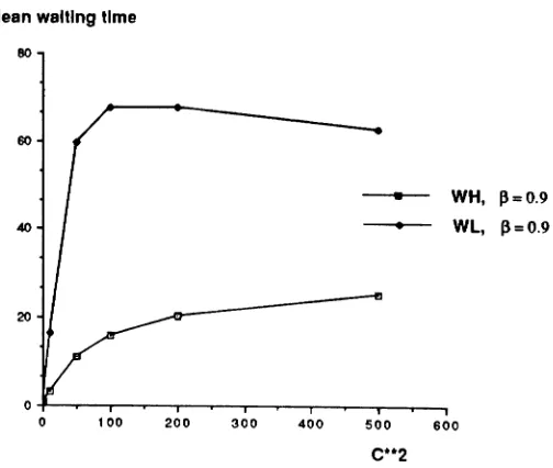
1. That is, during the busy period each slot contains a cell. We assume the same arrival process to each input line. Each arriving cell chooses one of the destination output lines randomly. The average utilization of the input line is 0.3. The results are summarized in Figure 7 to 16.

In Figure 7 to 9, (notated as WH and WL respectively) we plot the mean waiting time for both high and low priority cells with various

f3

values. The effect of C2

Mean waiting time

200

100 - WH, (3=0.8

- - + - - WL, 13=0.8

200 300 400 500

C**2

600

Figure 8: Mean waiting time for beta equal to 0.8.

Mean waiting time

80

100 200 300 400

•

•

500

C**2

WH, 13=0.9 WL, P=O.9

600

Mean waiting time of the high priority cells

30

20

10

--- C**2=1

- - - + - - C**2=10 --- C·*2=50

- - + - C**2=100 --- C**2=200

- - - 1 J - - C**2=500

1.0 0.8

0.8 0.4

0.2

o+---~--T---r-~----T----r...=...,---:;;.-.-r-=-~..;.---::_­

0.0

Figure 10: Mean waiting time of the high priority cells for various values of C**2.

Mean welting time of the low priority cells

300

1.0 0.8

0.6 0.4

0.2

oL~=*=::::;::t;~~::;::::;::;:::;::::::::~

0.0

&I _C**2=1

C**2=10

---

C**2=50

---+-- _C**2=100

C**2=200

200 ~ C**2=500

100

Mean waiting time of the high priority cells

30

20

10

•

WH, _tJ=0.9

..

WH, 13= 0.8

..

WH, 13= 0.7

~ _{WH, tJ=0.6}

•

WH, 13= 0.5

WH, f3= 0.4

•

WH, [3=0.3

•

WH, 13=0.2

•

WH, tJ=O.l

800 500

C**2

400 300 200 100

o~--r---..r-- --T""-r---r----T""-r---r--~-~...,

o

Figure 12: Mean waiting time of the high priority cells for various values of beta.

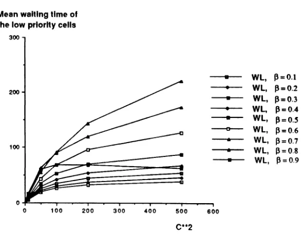
600 500 400 300 200 100

•

WL, f3= 0.1

200 WL, 13=0.2

•

WL, 13= 0.3

WL, 13=0.4

•

WL, 13=0.5

~ _{WL, 13= 0.6}

..

WL, f3= 0.7

100 _a

WL, 13=0.8

•

WL, [3=0.9

Mean waiting time of the low priority cells

300

C**2

Log(Prob. of Blocking)

o

-10

·20

-30

-40

- 1 ' - pbh, _P=0.9

- - a - - pbh, _P=0.8

- + - pbh, _13=0.7

~ pbh, _p=0.6

---

pbh, _P=O.S --.-- pbh, _P=0.4

- - + - pbh, _13=0.3

--+-- pbh, _fJ=O.2

---

pbh, P=O.l

-so

600

soo C**2

400

300

200

100

·60+--....~r--...---...,..-...-.-oop----.--.,...--...-....-....

o

Figure 14: Blocking probability of the high priority cells for various values of beta.

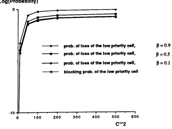
Log(Probebllity)

o

- - - + - probeof10••ofthelow prtorttycen, _____ probeof10••ofthelow prtortty cell,

- - - + - probeof10••of thelow prtortty cell,

---e-- blocking probe ofthelow priority cell

P=O.9

P=0.5

P=O.l

600 500

C**2

400 300 200 100

-10~-....-~-....-r--""'---,r---""""-""""''''''-''''-''''

o

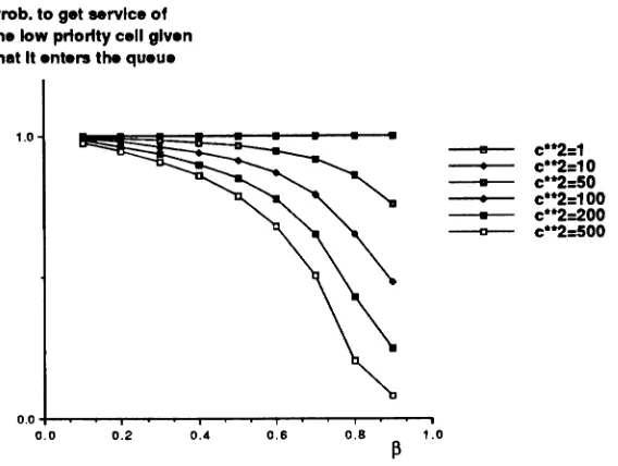
Probeto get service of the low priority cell given that It enters the queue

1.0

- - e - - c**2=1

- . - - c**2=10 - - c**2=50

~ c**2=100 - - c**2=200

- 0 - - c**2:S00

1.0

0.8

0.6 0.4

0.2

0.0+---...-....-...,....-~...----.

0.0

Figure 16: Probability to get service of the low priority cells.

7

Conclusion

Priorities and space preemption scheme were considered in a synchronous N x N Clos ATM switch with queueing capability at the input ports. The arrival process is modeled by an Interrupted Bernoulli Process. The cell processor queue was analyzed as an IBP

ICeol1

queue with finite buffer, head-of-the-line priority, and space preemption. Using the results from this queueing system, the ATM switch was then analyzed approximately.

References

[1] J.S. Turner "Design of a broadcast packet switching network", IEEE Trans. Comm. COM-36 (1988) 734-743.

[2] MJ. Narasimha"The Batcher-banyan self-routing network: university and simplification

", IEEE Trans. Cornrn. COM-36 (1988) 1175-1178.

[3] A.Huang and S. Knauer "Starlite: a wideband digital switch", IEEE GLOBECOM '84 Conf. Rec., 121-125, Nov. 1984.

[5]

F.~. ~obagi a~d

,;. Kwok "Fast packet switch architectures and the tandem Banyan

suiiichinq [abric ,Proc. NATO Advanced Workshop on Architecture and Perfor-mance Issues of High-capacity Local and Metropolitan Area Networks June 25-27 1990

S_oph· A_{ra- ntipo}· li_{s, France.} ' "

[6] S. No jima, et al. IIIntegrated services packet network using bus mairiz switch ", IEEE

J.

SAC SAC-5 (1987) 1284-1292.

[7] Y.-S. Yeh, M. Hluchyj, and A. Acampora" The knockout switch: a simple, modular

architecture for high performance packet switching ", IEEE J. SAC SAC-5 (1987) 1274-1283.

[8] H. Ahmadi, et ale "A high performance switch fabric for integrated circuit and packet switching", Proc. INFOCOM '88 (1988) 9-18.

[9] M. Devault, J .Y. Cochennec, and M. Servel "The 'Prelude' ATD experiment: assess-ments and future projects", IEEE Journal on Selected Areas in Communications YOLo 6, NO.9, 1528-1537,1988.

[10] II. Kuwahara, N. Endo, M. Ogino, T. Kozaki "A shared buffer memory switch for an ATM ezchange", Proc. Int. Conf. Communications (1989) 4.4.1-4.4.5.

[11] H. Suzuki, et al "Output-buffer switch architecture for asynchronous transfer mode",

Proc. Int. Conf. Communications (1989) 4.1.1-4.1.5.

[12] F .A. Tobagi "Fast packet switch architectures for boardband integrated services networks

", Proc. IEEE 78 (1990) 1133-1167.

[13] M.J. Karol, M.G. Hluchyj and S.P. Morgan "Input vs. output queueing on a space-division packet switch", IEEE Trans. Comm. COM-35 (1987) 1347-1356.

[14]

M.G. Hluchyj and M.J. Karol "Queueing in high-performance packet Bwitching", IEEE Journal on Selected Areas in Communications YOLo 6, NO.9, 1587-1597,1988.

[15]

Janak

H.

Patel "Performance of Processor-Memory Interconnections for Multiproces-sors", IEEE Transactions on Computers, VOL. C-30, NO. 10, October 1981.

[16] H.

Yoon,

K.

Lee, and

M.

Liu "Performance analysis of multibuffered packet-switching networks in multiprocessor systems", IEEE Transactions on Computers, VOL. 39, NO.

3, 319-327,1990.

[17]

S.Z. Shaikh, M. Schwartz, and T.H. Szymanski "Analysis, control and design of crossbar

[18] Y. Oie, T. Suda, M. Masayuki, and H. Miyahara "Survey of the performance of

non-blocking switches with FIFO input buffers", IEEE International Conference on Commu-nications VOL. 2, 737-741,1990.

[19] G. Hebuterne and A. Gravey, "A space priority queueing mechanism for muliiplezinq

ATM channels", Proc. ITC Specialist Seminar, Adelaide, Sept. 1989, paper 7.4.

[20] J. Garcia and O. Casals, "Priorities in ATM networks", Proc. NATO Advanced Work-shop on Architechure and performance issues of high-capacity local and metropolitan area networks, June 25-27, 1990, Sophia-Antipolis, France.

[21] , H. Korner, "Comparative performance study of space priority mechanisms for ATM

channels", Proc. INFOCOM '90.

[22] H. G. Perros "Performance issues in ATAf networks - A litterature review", Technical Report, Computer Science, NCSU.

[23] H. Heffes, and D. M. Lucantoni "A Markov Modulated Characterization of Packetized

Voice and Data Traffic and Related Statistical Multiplexer Performance", IEEE Journal on Selected Areas in Communications, VOL. SAC-4, NO.6, September 1986.

[24] A. A. Nilsson, F.-Y. Lai, and H. G. Perros "An Approximate Analysis of a Bufferless

Nx N Synchronous Clos ATM Switch", Proceedings, Canadian Conference on Electrical