Multi-attempt survey methods

,

(1

,

Charles H. Proctor

Institute of Statistics Mimeograph Series Number 2280 December 1995

North Carolina State University

Raleigh, NC 27695-8203

ABSTRACT

Surveys of households can be done by telephone or by mail or by personal

visit, while numerous calls or mailings or visits may be required' before getting

a response. If only one method is used and if an attempt is conducted i~ a

more or less standard way in all instances, then one can record results by the

number of attempts required and see whether there is a trend in the variable of

interest as more attempts have to be made. Such a trend can be used as a basis

to extrapolate to an unlimited number of attempts and thus to correct for

nonresponse caused by limiting attempts to just a few. We give details, for

the telephone survey case, of eight sets of model assumptions and how to decide

which one to work with. A further example of a mail survey is used to

illustrate estimation of a median.

The method is designed to furnish estimates of population proportions. The

population is defined as a large but finite realization under survey conditions

of values in a row by column array. The rows represent telephone numbers and

the columns represent minutes of the time period covered by the survey. The

notion of realization covers assignment of interviewer and other chance aspects

of the conduct of the survey. The values are whatever answer would have been

produced by calling that number at that minute. The values in any row are

called a temporal trajectory. Random numbers are used to select telephone

numbers and haphazard enumerator availability selects the times. These random

devices can then be expected to generate frequencies that will follow a

multinomial distribution. The population proportion, being one of the

parameters underlying this multinomial distribution, can thus be estimated.

1. INTRODUCTION

The method being considered here was introduced in an earlier, rather

wide-ranging, paper dealing with case nonresponse (Proctor 1978). Its possible

application to telephone surveys was mentioned there, but not explored

extensively. We propose here to consider more details of the telephone survey

'setting and to suggest how the m~thod might fit into current practices. In

brief, the method involves calling a random sample of telephone numbers and

setting a rather low maximum number of callbacks -- for example, three calls.

Data obtained from telephone conversations on the variables of interest are

tabulated separately by call. Whatever association exists between no-answer

proportion and level of the variable can thereby be detected and corrected by

extrapolating to a larger number of calls. We also illustrate how the method

cou1~ be used to estimate a median in a survey by mail. This second example

shows the method's flexibility.

It may be helpful at the outset to alert readers that using the method will

require strict adherence to uniformity of approach by the enumerators. While

an enumerator will choose when to signal readiness to make a call, the

telephone number to be called will be furnished at random from those in the

sample to be called. The probabilities in the model derive from the random

number tables and so long as the random numbers are honest and the enumerators

adhere to instructions the model will be correct.

It was in such a finite population setting that Deming (1953) noted the

serious biases that could arise from failure to obtain a response to mail and

'.

provided by Walter Hendricks (1949) might be adapted to reduce the bias by

developing some "new type of estimate." This is essentially what the method of

this paper affords.

Among the methods for handling case nonresponse that Cochran (1977)

reviews, all seem to have certain operational drawbacks. The Hansen-Hurwitz

(1946) follow-up method draws a subsample of nonrespondents to a first attempt

and subjects this relatively small group to whatever extensive effort seems to

be be needed to secure a response. The drawbacks are the possibility of

distorting the response by the effort required and the possibility of failing

to get a response even after expending the effort. When carried to a

successful completion, however, the estimate is unbiased.

Other methods such as recording times-at-home for use in weighting factors

(Politz-Simmons, 1949) or doing just one callback with a "level playing field"

by finding out for everyone when they are likely to be in (Bartholomew, 1961)

depend on a degree of careful and truthful information being provided by

informants that informants don't uniformly provide.

Other methods such as reassigning for interview in the present survey cases

found to be case nonrespondents in earlier surveys (Kish and Hess, 1959) or

using herculean efforts to reduce nonresponse (Dillman, 1978) are certainly

going to reduce bias, but it is difficult to know by how much.

In my experiences with application of the multi-attempt approach the main

difficulty was getting enumerators, or perhaps it was supervisors, to accept

reassigning the telephone numbers to enumerators for each attempt. I'm not

sure what is the source of the resistance. Perhaps the numbers could be dialed

of waiting 5 minutes, then dialing again when a busy signal is detected, could

also be incorporated into the attempt [see Groves and Lyberg (1988)]. Certainly,

by varying the calling times one may be able to increase somewhat the answering

rate, but this will come at the price of an unknown amount of bias. The size

of the bias is quite likely small, but not knowing it is unacceptable -- at

least I would find it so.

2. MULTI-ATTEMPT TELEPHONE SURVEY METHODS

The enumerators of the telephone survey are to make their calls with

temporal spacings entirely dictated by their convenience. The telephone

numbers they dial will be randomly assigned to them at each call without regard

to who the enumerator is or to any other features. Suppose that four calls

(r=4) is decided on. The n sampled numbers will all be called in some random

order. The no-answers will be randomly reordered and all called. The

remaining no-answer numbers will again be reordered randomly and all called and

finally the three-time no-answers will be randomly reordered and called a

fourth time, again in that re-randomized order. If, at any call, the

enumerator arranges to call again at a more convenient time, the follow-up call

is still considered part of the initial contact. If refusals are turned over

to a supervisor who attempts to convert them to responses, the final result is

attributed to the contact of the refusal.

The observed values obtained from the telephone conversations can be such

categories as "one household member says Yes and two say No" or "one male of 35

years, registered to vote, and one female of 7 years." The survey objective

such proportions can be furnished with an estimated covariance matrix and thus

standard errors for estimates of conditional proportions or of medians or of

other parameters based on the proportions can be calculated.

3. POPULATION NOTATION

The population subject to survey will be represented by a collection of all

possible telephone numbers, with each having its temporal trajectory. The

temporal trajectory of the ith number is denoted Yi(t) where t indexes, from

*

t = 1, to t = T , all the minutes of those days during which the survey is

being carried out. In general, Yi(t) for a given i will be a sequence of

recorded values of the survey variables that would be obtained if a call to the

*

ith telephone number were made at time t, for t

=

1, 2, ... , T. For

illustration, consider the following possible values of Yi(t).

Yilt) = "~," or not working, if the manner of ringing or a recorded

message from the telephone company indicates that the number is not

connected.

= "A," or no answer, as when 10 rings go by, an unconverted busy

signal sounds, or an answering machine comes on.

"R" if a refusal is encountered.

"E" if the number is ineligible or not a member of the population

of interest (such as a business if the survey is of residences).

= "aN" or someone answers "No" to the survey's query.

"aU" or someone answers "Undecided."

In most surveys it is possible to ignore the Q's and we will do so here.

In this example there are five possible values of Yi{t) aside from

A.

In the

general model below, K= 5 and k indexes these categories.

If there are N possible working telephone numbers that can be dialed and if

*

*

there are T minutes that are subject to survey, then NT is the size of the

finite population subject to survey. That is, each value of each trajectory

may be considered a separate population value. It is usually recognized that

the proportion of refusals and of item nonresponse, as well as respondent

burden, is likely to be high at nighttime and even in the mornings, so that a

decision may be made to make calls only during certain most propitious times of

certain non-holiday and non-weekend days. Let there be T such minutes during

which the enumerators are working. The NT values of Yi{t) are the surveyed

population.

Temporal trajectories, Yi{t), will be found to be a helpful conceptual

device, although it is difficult to see how to establish them empirically in

all their detail. Which people are at home at various times determines to a

great extent when

A

or R or even which answer will be recorded. The

quality of interviewing and the care with which questions are worded, in

particular, who is the enumerator, will determine ,the consi$tency of aY, aU

and aN through time. We can see that it would require careful questioning to

determine a complete temporal trajectory for anyone telephone number. There

are, however, many global features of such trajectories that can and probably

should be investigated. Recording time of call, by which enumerator, along with

the response, for example, could be made a routine feature of multi-attempt

reinterviewed, by a different or by the same enumerator, to ascertain response

consistency. This kind of information is, however, entirely inessential to the

operation of the multi-attempt method.

Notice that both the Yi(t) as well as the "stable" values, Yi(u) to be

defined below, are all random quantities. They are drawn from a hypothetical

infinite population of survey realizations, or, to be a bit more explicit, of

equivalent complete coverages. We may denote by ~ the parameter of interest

calculated from, say, the Yi(u) -- from all N of them. Let's say ~ is the

proportion of aV's among these N quantities. A given realization would pair

certain enumerators with certain telephone numbers, while eventually, over all

possible realizations, all enumerators would appear as having worked on all

telephone numbers. Considering the huge sizes of T and of N it is usually

clear that any particular ~ will be extremely close to E(#) where the

expectation is taken over all realizations.

A crude upper bound on the difference between a proportion # and its

expectation over realizations, E(#), can be computed as /1/4N. Even when N

counts only working numbers rather than all possible numbers, this difference

should be found to be inconsequential in practice. Derivation of this bound

may aid in understanding the method. The following illustration is constructed

with unrealistically small values for T and N so as to increase the realism.

Suppose the population to be surveyed is one exchange of 10,000 numbers,

and the time is one day from 2 p.m. to 8 p.m., so T = 360. Further suppose

there is a staff of 100 enumerators working at consoles during the survey.

Randomly permute the 10,000 numbers and as the enumerators signal they are

different realization would be obtained from a different permutation. If all

that is recorded is:

A

= no answer, aM = voice answering is judged as male

or aF

=

voice answering is judged as female, then diligent enumerators may

manage to get through all 10,000 numbers. We will suppose they did.

The ,proportion of aM among the 10,000 observations essentially constitutes

,~. Actually only 1/360th of the population values have so far been obtained so

the real ~'s will be somewhat less variable than the proportion (say

y)

based

on the 10,000 calls. For purposes of an upper bound we may roughly suppose the

10,000 observed values (the Yi say) were generated by an additive variance

components model as:

y.

=

~ + a. + ~. + e.·

1 1 J lJ (3.1)

where ~ is a grand mean, the ai's are household (telephone number) effects, the

~J"s are enumerator effects and e .. are enumerator by household effects. lJ

The total variance (say a;) as well as the variance components (say

a~,

a~

and

a~)

are each bounded above by .25

=

1/4 since the range of Yi is from

zero to one and none of the component's range would dare to exceed this. In

fact we would definitely expect a~ to exceed zero and for most collections of

enumerators so would a~. A crucial finding is that, as realizations are

varied, the a_i and the ~j stay roughly constant. That is, the

P

_j are

enumerator biases and, although a particular run of easy or difficult calls may

jar this bias a bit, it will not be much. The ai's derive from the single

person households and others in which answering the phone is assigned to one

person. Thus V(y) =

a;/N,

and V(y) « 1/4N, giving the above mentioned

Oftentimes, there is a preferred method of measurement. It may involve

record checks with personal visits and so forth. Let the parameter of interest

when calculated from results of preferred measurement methods be denoted p'.

If the survey measurements are biased then this will produce discrepancy

between p and p' .

It may also happen that the collection of persons reached through the N

telephone numbers is larger or smaller than some collection of persons of

interest. The survey times may also exclude nighttime hours that if included

might reduce the cases of YilT) =

A.

We will define the quantity p" to

include the notion of coverage of the so called target population as well as

use of the preferred measurement method. Thus the difference (p' - p) will

reflect measurement bias while (p" - p') will represent coverage bias. These

notions are introduced just to make clear the limitations of our multi-attempts

method. It will not solve measurement biases nor coverage problems.

4. ASSUMPTIONS OF THE METHOD

A population parameter of interest could, perhaps, be described as the

proportion of aV's, among the NT values of Yilt), but .some care needs to be

taken here. One might suggest defining a summary value for each telephone

number depending on which value predominated over the survey period. These

values would constitute the vector Yi(a), say (with a standing for "stable").

Notice that there will also be some Rand

E

values among the YilT), as well

as some A only. Another approach would be simply to use the eXisting

proportions of aY's, of aU's, etc. over the survey period as the summary

values for the number. The vectors of proportions may be denoted Y.(T) where

each vector has K components. The K proportions based on the Yi(u) should be

very close to the means of the Yi(1). A third, rather refined, approach would

be to define the summary variable to be just aY, aN or aU, but to use any

time trend there might be in the trajectory to predict the answer which would

predominate in the month following the survey period. These quantities may be

denoted Yi(n), say (with n = "projected"). We anticipate that the differences

among such alternative population parameters would be insignificant in any

practical sense, although it is also important to be aware of possible

exceptions.

For simplicity's sake we will suppose responses for anyone trajectory are

all aY, all aN or all aU. We also suppose a refusal for i will be a consistent

case of Yilt) = R for all t, and

E

will also be consistent except when

Yilt) = A, of course. Remember there may still be some A-only cases, the

hard-core no-answer. The outcome of the survey, i.e., how many respond at

each of the contacts and what they say, is determined basically by the

differing relative frequencies of A's to answers among the Yilt) values. One

would ordinarily expect these relative frequencies not to change in any

systematic way during the survey period. It will happen, however, that the

telephone numbers with the relatively more inaccessible aN's and aU's and aY's,

as well as E's and R's will be called more often as later waves focus on

nonresponders, and this will be taken into account.

The time from t = 1 to t =T

1, say, during which all n first attempts are

made will be denoted the first-calling period; that from t = T₁ to t

=

_T2

during which a second call is made to the no-answers is the second calling

proportions of A within the periods and this would not upset distributional

assumptions sin~e the random reordering of numbers assigned to be called will

overcome this. If there are a few degrees of freedom left over from fitting

the observed frequencies to the theoretical ones, departures from such

assumptions can be detected if they are pronounced enough.

The many idiosyncratic events occurring to the enumerators, along with the

random ordering of the numbers to be called, should insure that the actual

times the calls are made will be roughly uniformly distributed over the

surveyed times -- as well as equally distributed over the numbers for that

wave. Both the total number of times T and the number of telephone numbers N

are finite and thus, although we will be supposing the observed frequencies to

have a multinomial distribution, the actual distribution is multivariate

hypergeometric. The number of minutes in an interval, even in the last calling

period from Tr -I to Tr , will generally be so large as to be effectively

infinite. For example, in one month there are about 10,000 survey minutes.

Sample sizes in most telephone surveys are but a very small proportion of the

working numbers and so finite population correction factors (fpc's) will not

be needed for N either. Since the actual population being sampled has TN

values there will be no' need to use an fpc.

Let PIN be the population number of telephone numbers giving the answer

aY, or "Yes," as based on Yi(a). Also, suppose that Q

I is the proportion of no-answers (A's) among the PINT values of their corresponding Yilt) quantities.

Similarly, we define P₂ with Q

2 and P3 with Q3 to refer to those answering

"Undecided" and "No," respectively, while P₄ with Q

4 and P

s

with QS refer to

say, is greater than zero, then there is a proportion 1 of numbers that are

consistent no-answers. The presence of nonworking numbers among the 1N can be

a problem, since a number where no one is ever at home during the survey period

cannot be distinguished from a not-connected number that rings normally.

5. MODEL EQUATIONS

The observed frequencies appear as in the Figure for a case where the

variable of interest is a trichotomy. Let us suppose the population number of

nonworking numbers is indeed known and our initial sample was of size n_I. We

can thus ignore the number of known nonworking numbers and deal with a sample

of size n = nI - nW'

The population can now be visualized as an N by T matrix with entries aV,

aU, aN, t, R or

A.

In a given row all non A's are the same and are

equal to Yi(a). The data collection process begins by the random selection of

a sample of n rows, say i 1i2... in' from the N. Next a selection of n times

(columns) t₁ < _{t 2} < ... < _{t n is made in the interval 1 to t n}

=

T₁, and finally

a random permutation of the selected n rows say i(I), i(2) ... i(n) is merged

with the times and the values Yi(£)(t£), 1 = 1, 2, ... , n are recorded. From

these data the frequencies in Figure 1 can be obt~ined by tally.

It should be clear by now how the realism of a multinomial model for the

frequencies depends not only on the honesty of the random numbers used to

sample rows (telephone numbers) but also on the independence of selections of

columns (times) from selection of rows achieved by random ordering of the

numbers to be called.

In a preliminary fashion we first suppose that, in any row where Vi(a)

=

the

underlying the frequency at the jth attempt in response category k, k

=

1, 2, ... ,

K, is then given by the expression:

(5.1)

Although this multinomial model provides an interesting special case, it will

be strictly correct only if all trajectories in category k have a_{k as their}

proportion of A's.

In order to accommodate to some heterogeneity of trajectories, _{ak will be}

replaced by a three-point distribution with probabilities, W, 1-2W and Won

corresponding values a

k - A, ak and ak + A. Now (5.1) can be extended to:

The value of A is set as the minimum, over k, of the smaller of .95a_k or .95(1-a_k).

The quantity .95 has been varied from .50 to .99 for a number of examples and

the estimates appear to be unaffected.

The probability underlying the number of no-answers at the last call is just one

minus the sum of probabilities in (5.2), namely

(5.3)

There are Kr+l observed frequencies and, in addition to the value of n, there

are 2K+l parameters (K a's, (K-l) P's, 1 and W) to use in fitting to the

frequencies. Any method for fitting a multinomial model that seems convenient

may be used. The results should include estimates of the parameters, a

goodness of fit statistic, an estimated covariance matrix for the parameter

6. CALCULATION PROCEDURES

The program that was used in the following examples does iterative fitting

to a multinomial model in accord with Fisher scoring. First derivatives of the ~jk

are calculated :lumerically -- adding and subtracting 10-5 from each parameter

yalue in turn and then 'multiplying the difference in proportions from (5.3) by

5 x 104. Starting values for the class proportions are obtained as observed

proportions after pooling the data over all calls. The corresponding starting

values for nonresponse proportions come from the ratio of class frequencies at

the second call divided by those at the first call.

Let's just outline the basic calculations to be programmed, and for

simplicity we take the case where Whas been set to zero. Start with a column vector of (rK+1) observed frequencies,~. Put the probability quantities, the

n_j , in the {rK+1)-by-1 column vector~. Their first derivatives appear in the

(rK+1)-by-2K matrix

o.

The 2K parameters are in 8. The efficient scores are

obtained as s = (n #/n)'O where "#/" means to divide termwise. The entries of

the information matrix B are obtained as

(6.l)

where d_i and de are columns of

o.

The inverse of Bbecomes the covariance matrix V B- 1.

We use the superscript (m) to refer to the mth step of iteration. For the

starting values one uses m=

o.

We have already described how to obtain 8(0) and thus how to calclJlate ~(o), 0(0), s{o), B{o) and V{o) . The mth iteration step

o(m) = O(m-I) + V(m-l)

*

s(m-l) , m= 1, 2, ... , M • (6.2)

The iteration proceeds until O(m) and O(m-l) agree as closely as machine

rounding allows. Say this occurs at the Mth iteration.

A goodness of fit statistic, say X2; is calculated by squaring and adding the

quantities:

(6.3)

which are themselves a species of standardized residual and can serve to point

to lack of fit of various types. The statistic X2 is referred to the

chi-squared distribution on K(r-2) degrees of freedom. The diagonal entries of

V(M) are estimated variances of the parameter estimates.

Suppose we denote the first K entries in O(M) as PI' P2' •.. , PK' and also

suppose there is interest in the estimate PCl

=

Pl/(PI + P2 + P3)' In our

example, this is the estimated proportion of Yeses among Yeses, Undecided and

Noes. To find an estimated standard error we extract the upper-left 3-by-3

submatrix of V(M) -- as VI say. Next compute a 3-component coefficient vector

C with entries the derivatives of PCl: (PI - l)/(Pl + P2 + P3)' Pl/(Pl + P2 + P3)

and Pl/(Pl + P2 + P3) and finally calculate C'VIC as an estimated variance for PCl'

7. NUMERICAL ILLUSTRATION

The following data are from a telephone survey that was done to inquire

about the effects of 4-H club membership among the US adult population. The

sample of telephone numbers was furnished by a survey research firm, Survey

Sampling, Inc., and the interviewing and tabulations were done at Texas A and M

statistical con5ultant. Three telephone attempts were made and the telephone

numbers were re-randomized among interviewers at each calling.

Before examining the responses to the various questionnaire items we first

looked at a basic three-way breakdown into Refusals, Non 4-H households, and

4-H households by the three calls. This was done separately by four regions of

the US. There were sizeable differences in parameter estimates among the

regions. The frequencies and parameter estimates are in Table 1 while fit

statistics are in Table 2.

Each set of frequencies is fit by eight models, designated as Model 1 to

Model 8. The first four cases use a single response propensity, while the last

four permit a separate response propensity (Qk) for each category. Models 1 and

2 as well as Models 5 and 6 set the proportion of consistent no-answers equal

to zero (1 = 0) while the other four models permit there to be some such. The

odd numbered models have the heterogeneity weight set at zero (W=O) and the

even numbered ones permit the three-point distribution of response propensity.

The chi-square goodness of fit statistics for each model and for the four sets

of data appear in Table 2. The results show that Model 6 with heterogeneity

but no consistent no-answers fits the best. We may believe there to be a few

consistent no-answers but getting a reasonable fit with Q = 0 suggests there

are only a few.

It can be seen from the fit statistics, and also from common sense, that

the assumption of response propensity heterogeneity is an alternative to the

assumption of the presence of consistent no-answers. That is, the presence

call to call. The presence of heterogeneity implies that the relatively more

accessible cases will respond earlier and that later calls will also see a

declining response rate. This relationship of alternatives between the two

parameters explains the poor showing of Models 4 and 8 in which both parameters

are allowed to va~. ' It may happen that one parameter is forced to its lower

boundary at zero. Our program shows poor fit whenever this occurs. It, also

may occur that a locally best fit inside parameter space may turn out not to be

as good as one on a boundary.

Notice in Table 2 the higher no-answer propensity among the Refusals than

among the Non 4-H in all regions and also among the 4-H members in the South

and Northeast regions. Heterogeneity is highest in the North Central and

lowest in the South Region. These findings are consistent with the nature of

regional differences that I would have expected. People who are harder to

contact may well be found in greater abundance among the refusers. Heterogeneity

is a mark of there being some appreciable number of always-answer cases as well

as fairly frequent never-answer cases. The South tends to avoid these

extremes. I visualize more housewives there but they are not always at home.

Although these findings are encouraging for the reasonableness of the

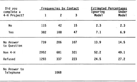
model they were not the'purpose of using the method. Our real interest was to

correct any bias in estimated proportions of questionnaire item response. The

frequencies in Table 3 and 4 show two of these items and th~ proportions are

estimated both by applying the model (Model 6, that is) estimates of response

propensities and also by ignoring such differences. , The main finding is how

little difference there is between the raw sample percentages and the model

These results also serve to point out where are the major difficulties

caused by no-answering. The refusals and the did-not-answer-the-question cases

are numerous and are projected to be relatively a bit more numerous if calling

was to continue forever. About 27% of the called telephone numbers would

produce refusals and about 15% would not answer these questions. The

smaller, sample unadjusted percentages corresponding to these two are 24% and

14% so, even here, the change is relatively small. These findings of small

biases (if a 1% or 2% change can be called "small") are most welcome for this

survey since expanding the sample cases to give population estimates will be

tedious enough without having to carry along a correction for noncontacts.

If biases due to nonanswering cases are, in some survey, found to be rather

pronounced and the sample is from a complex design, then we would suggest

incorporating a simple multiplicative adjustment to the raising factors.

That is, each observation would be carrying whatever raising factor (or weight)

is needed to reflect the sample design. The additional multiplier would be

computed as the ratio of the estimated percentage from the model to the

percentage based on sample unweighted frequencies. Consider as an example the

conditional percentages for the first three answer categories for question 2G2

of Table 4. The model percentages would be 10.5, .35.4 and 53.1 with sample

percentages of 11.8, 33.3 and 54.8 so the multipliers are .89, 1.06 and .97.

These would be applied to the sample design raising factors to get the final

raising factors. Notice that the adjustment applies only to the one item. To

adjust a cross classification one would obtain separate multipliers for each

8. SECOND ILLUSTRATION

The following case illustrates a use of the multi-attempt model in the

sample design phase of a mail survey that also involves a parameter other than the

basic proportions. In studies of ratios of the recorded value of taxable

property to sale value there is interest in the median of the distribution.

The median is a reasonable choice of central value here in view of the rather

extreme swings that can be seen in this ratio. The model of multi-attempts can

be used to estimate proportions in classes of the ratio. The median would then

be calculated by straight line interpolation from the estimated cumulative

distribution function, while the standard error of the estimate can be judged

from the covariance matrix of the class proportions.

From past experiences, it was judged that nonresponse propensities of 80%

or 90% would not be unusual. A survey form is mailed to a sample of business

addresses and just the goodwill of the business determines if there will be a

forthcoming report on any sales of taxable property items. We also introduced

some inequalities in these propensities and furnished some evidence of a

slowing down of response rate by mailing. For a mail survey an attempt is

called a mailing and is defined by a time period such as three weeks.

Addresses not returning in three weeks are sent another questionnaire. Our

hypothetical data are in Table 5, where the total sample size was taken to be

1000. Class limits would generally be chosen so that the median falls into a

rather narrowly defined middle class, while the other two proportions would be

If the class limits are denoted a and b while the proportions are PI' P 2, and I-PI - P2 ' then the estimator of the median is

(8.1 )

From knowledge of the variances and covariances of the estimated proportions we

,can obtain, from a Taylor's series expansion, a variance for M. For the

normal distribution and random sampling this variance is found to be (wu2/2n).

The distribution of rat i os wi 11 be fairly well approximated by the normal in

A A

the neighborhood of the median. The variances of PI and P₂, however, will

not be given by the familiar "pq/ n" formula as for random sampling, but will be

given by the multi-attempts model. In the random sampling or binomial case one

should perhaps use, as a value of sample size, the number of responses, which

is 257 in our example, rather than the initial sample size of n

=

1000 in our

example.

When Model 6 is fitted to the data of Table 5 the estimated variances for

A A

PI = .432 and P₂ .417 are .000953 and .000946 respectively. The

corresponding pq/n quantities with n

=

257 are .000955 and .000946 which shows

an almost exact agreement. The unadjusted proportions are PI = .230 and

A A

Pz

.486 so the estimates PI = .432 and P

2 = .417 would be expected to be

less biased. When Model 8 is fitted then the estimated proportion of hard core

nonrespondents is .09 and there may be some question as to the presence of such

cases.

Judging from past experiences we can expect the standard deviation of the

central or non-outlier distribution of ratios to be about 50% of the median

itself. This implies a 4% sampling coefficient of variation for Min the

S~~~~

= Sample CV of M= Population CVJw/2n

=

50Jw/2 x 257

= 3.9

A most conservative viewpoint on the 9% of hard core nonrespondents would be to

suppose they would all be above or all be below the observed median.. This

proportion (1 = .09 in this case) could affect the position of the median by the

amount 1~ a or, relative to the median itself, by 1~ x 50% K 11.3%. Notice

that this latter uncertainty is most unpalatable in that it does not diminish as

sample size increases, as well as being three times larger than sampling

uncertainty.

9. PARTING COMMENTS ON EFFICIENCY

In the 4-H survey cited above three attempts were made. This is the

minimum number required in order to estimate the parameters of the model.

Whether three or four or even more attempts should be made depends, of course,

on survey costs and on the model parameters. As in many such problems of

sampling design the optimum is flat. For example, four attempts may give least

variance for fixed cost but three or five or even six, seven, or eight will not

be much worse.

To illustrate these considerations we used the parameter estimates for the

data in Table 3 to project what would have been observed if four attempts had

been made. From these projected frequencies it can be determined that a sample

of size 8306 with four attempts rather than the actual 8636 with three

REFERENCES

Bartholomew, D. J. (1961). "A method for allowing for 'not at home' bias in

sample surveys," Applied Statistics, 10:52-59.

Cochran, W. G. (1977). Sampling Techniques. Third Edition, John Wiley and

Sons, New York NY.

Deming, W. E. (1953). "On a probability mechanism to attain an economic balance

between the resultant error of response and the bias of nonresponse,"

JASA 48:743-772.

Dillman, D. A. (1978). Mail and Telephone Surveys: The Total Design Method,

John Wiley and Sons, New York, NY.

Groves, R. M. and Lyberg, L. E., Chapter 12, Groves, R. M., et al., Editors,

Telephone survey methodology. John Wiley and Sons, New York, NY, pp. 191-211.

Hansen, M. H. and Hurwitz, W. N. (1946). "The problem of nonresponse in

Hendricks, W. A. (1949). "Adjustment for bias by nonresponse in mailed

surveys," Agricultural Economics Research 1:52-56.

Kish, L. and Hess, I. (1959). "A 'replacement' procedure for reducing the

bias of nonresponse," American Statistician, 13(4):17-19.

Politz, A. N. and Simmons, W. R. (1949). "An attempt to get the 'not at

•

homes' into the sample without callbacks," JASA 44:9-3l.

Proctor, Charles H. (1978). "Two direct approaches to survey nonresponse:

estimating a proportion with callbacks and allocating effort to raise

response rate," in Proceedings of the Social Statistics Section - American

Figure. Notation for Frequencies and Population Parameters

Known Not Undeci- Not

No-Call Working Yes ded No Refysal El ig1 bl e Answer

1 n

_W

n_{U nI2 nI3 n14 n15 n16}

•

2 0 n2I n22 n23 n24 n25 _n26

r 0 nrI nr2 nr3 nr4 nr5 nr6

Population Proportions PI

No-answer Proportions a

Tabl e 1. Sample Frequencies by First, Second or Third Attempt for Three Basic Types of Answer to a Telephone Interview with Parameter Estimates

for a Model of Multi-Attempt Surveys

Parameter Estimates

Sample Frequencies No-answer

Telephone by Attempt Estimated Proportion

Hetero-•

Answer Percent, A geneity

Type 1 2 3 100Pk tr

k Weight, W

Northeast

4-H 253 74 48 23.3 .52

Non 4-H 813 170 95 51.3 .30 .23

Refused 344 98 54 25.4 .39

No Ans. 292

South

4-H 292 115 57 27.9 .50

Non 4-H 617 156 90 43.9 .35 .15

Refused 339 89 76 28.1 .45

No Ans. 294

North Central

4-H 383 79 33 24.1 .27

Non 4-H 755 158 73 48.8 .29 .31

Refused 312 83 48 27.0 .45

No Ans. 238

West

4-H 308 88 31 22.1 .33

Non 4-H 767 197 63 51.6 .29 .25

~)

Refused 298 67 45 26.3 .48

Table 2. Fit Statistics for Eight Models Fitted to Data of Table 1.

Case OF Northeast South North Central West

1 6 164.6 106.3 178.6 152.0

•

W '" 0 2 5 16.3 29.3 9.4 14.1

Equal

Q _{"( '" 0 3} 5 57.0 . 53.5 42.8 23.0

"( t 0; _{W '" 0 4} 4 193.7 247.6 9.4 11.7

5 4 106.0 82.8 108.4 115.2

W '" 0 6 3 11.9 22.9 2.2 6.1

Unequal

Q

"( '" 0 7 3 43.6 42.7 30.5 16.4

W '" 0; "( '" 0 8 2 64.1 145.4 8.9 6.4

Sample Size 1141 2125 2162 2108

Table 3. Responses to Question 20 by First, Second or Third Call

Did you Frequencies by Contact Estimated Percentages

complete a Ignoring Under

4-H Project? 1 2 3 Model Model

No 115 42 15 2.3 2.3

Yes 382 108 47 7.1 6.9

No Answer 739 206 107 13.9 14.5

to Question

Non 4-H 2952 681 321 52.2 49.1

Refused 1293 337 223 24.5 27.2

No Answer to

..

Table 4. Response to Question 2G2 by First, Second or Third Call

Rate Usefulness Estimated Percentages

of Your Experi- Frequencies by Contact

ences with Ignoring Under

People in 4-H: 1 2 3 Model Model

Some 64 12 8 1.1 1.1

Useful 160 55 23 3.1 3.4

Extremely 273 83 31 5.1 5.1

Question Not

Answered 739 206 107 13.9 14.8

Non 4-H 2952 681 321 52.2 49.4

Refused 1293 337 223 24.5 26.3

Telephone

Table 5. Hypothetical Data for Planning a Survey to Estimate the Median of Ratios

Estimated Parameters for Case 6 Model

Contact A

C1 ass Limits _{Pk ak} W

•

1 2 3

Zero to a 21 20 18 .432 .951

a+ to b 50 40 35 .417 .881 .226

b+ 35 20 18 .152 .779