ABSTRACT
NIKAS, ARIEL NICHOLE. Morphoelastic Modeling Applied to Stomach Bending and Lung Branching. (Under the direction of Sharon R. Lubkin.)
Morphoelasticity, an emerging area of continuum mechanics, can describe the large strains of
organogenesis. This framework multiplicatively decomposes the deformation gradient tensor into a
growth tensor and an elasticity tensor that ensures compatibility. We apply this framework to two
systems, lung branching and stomach bending.
In the embryonic stomach, the curvature changes as the stomach develops and the stomach
shape becomes LR asymmetric. However, the emergence of the asymmetry in the stomach during
organogenesis is not well understood. Recent experiments have shown that asymmetrical gene
expression in some way causes this bending rather than external forces or rotation. We modeled
several different types of growth using nonlinear solid mechanics to test hypotheses on the cause of
stomach bending. In this thesis, we ruled out a greater rate of overall mitotic growth on the left as
the cause for asymmetry in the stomach. Rather, we found that anisotropic growth, representing
different oriented cell rearrangements or divisions, is necessary to obtain the shape changes seen in
the developing stomach. Specifically, increased axial lengthening combined with radial thinning on
the left side create a shape change most similar to published experimental studies.
Many previous models of lung branching morphogenesis were focused on the complex
mor-phogen signaling systems and either omit explicit modeling of shape change, or model shape change
by moving a surface normal to itself without explicit mechanics equations. Previous models have
shown that morphogen flux distribution corresponds to the location of branching, and that this
distribution is reliant on local geometry. In this dissertation, we explicitly modeled both the
mor-phogen signaling and the resulting growth dependent on the calculated mormor-phogen flux distribution,
in a novel application of morphoelastic shell modeling for lung growth. We concluded that local
geometry affects the resulting shape change. Specifically, we observed tubule lengthening for all
the thickness of the epithelium affects the resulting shape change. These two different modeling
approaches of solid mechanics and shell mechanics combined with morphoelasticity allowed us to
© Copyright 2019 by Ariel Nichole Nikas
Morphoelastic Modeling Applied to Stomach Bending and Lung Branching
by
Ariel Nichole Nikas
A dissertation submitted to the Graduate Faculty of North Carolina State University
in partial fulfillment of the requirements for the Degree of
Doctor of Philosophy
Applied Mathematics
Raleigh, North Carolina
2019
APPROVED BY:
Mansoor Haider Nanette Nascone-Yoder
Ralph Smith Sharon R. Lubkin
DEDICATION
To Watson Nikas. You walked across my keyboard while I was applying to graduate school and you
BIOGRAPHY
The author was born in Maryland in 1991. Ariel competed in timed hard drive replacing, which
explains a lot. She then attended Meredith College in Raleigh, North Carolina where she graduated
with a B.S. in mathematics. During her time at Meredith, she also earned a black belt in aikido. Later
ACKNOWLEDGEMENTS
This work would not have been possible without the support of many people. I would like to thank
my advisor, Dr. Sharon Lubkin, who listened to many wild speculations, read too many drafts, and
always had a good story. I would also like to thank my committee members, Ralph Smith, Mansoor
Haider, and Nanette Nascone-Yoder, who taught me to model and ask questions. None of this could
have been done without the patience and kindness of many people from the department, especially
the assistance of Di Buckland and Carolyn Gunton.
This work would not have been possible to complete without support from the CRSC at North
Carolina State University and Dr. Hien Tran.
I would like to thank all my Meredith College math professors, especially Dr. C. Manning who
supervised my undergraduate research and got me started on this path and Dr. Hontz who taught
the majority of my math classes and was always available for advice. I appreciate your belief that I
could do this.
Thank you to my family for feeding me, watching too much of The Hobbit, and randomly handing
me avocados to go home with.
Of course, I would like to acknowledge Travis Rhea who did too much to detail in any way that
represents the actual amount. Thank you for the love and support and for never giving up on me
even when I was delirious from lack of sleep, and always being down for taco Tuesday.
Thank you to the McElroy brothers Justin, Travis, and Griffin who were full of advice for the
modern era but also goofs. This degree does not make me a doctor of "horse-bone-ology."
I would like to thank all the cats I have lived with over my time in graduate school, my beloved
Watson Nikas, Burton Guster Nikas-Rhea, Oxford Nikas-Chaney, Dr. Pep Pepterson Thomas, Pudlet
Thomas, and Thea Noorman.
And of course to my wonderful fellow graduate students, Emma Sorrel, Ben Randall, and Evan
TABLE OF CONTENTS
LIST OF TABLES . . . vii
LIST OF FIGURES. . . .viii
Chapter 1 Overview . . . 1
1.1 Organ Morphogenesis . . . 2
1.1.1 Stomach Organogenesis . . . 3
1.1.2 Lung Organogenesis . . . 4
1.2 Morphogenesis Modeling Overview . . . 4
1.2.1 Agent-based Modeling Approaches . . . 5
1.2.2 Continuum Modeling Approaches . . . 5
1.3 Isotropy, Anisotropy, and Inhomogeneity of Growth . . . 6
1.4 Mathematical Background . . . 8
1.4.1 Morphoelasticity . . . 8
1.4.2 Continuum Mechanics . . . 16
1.4.3 Hyperelasticity . . . 18
1.5 Summary of Morphoelastic Framework . . . 21
Chapter 2 Details of Mechanics. . . 24
2.1 Solid Mechanics . . . 24
2.1.1 One-Dimensional Example . . . 26
2.1.2 Three-Dimensional Example . . . 27
2.2 Shell Mechanics . . . 29
2.2.1 General Shell Theory . . . 32
Chapter 3 Implementation & Verification . . . 37
3.1 COMSOL Implementation . . . 37
3.1.1 Implementing Growth . . . 38
3.1.2 Local Coordinate Systems . . . 39
3.1.3 Hyperelasticity . . . 42
3.2 Model Verification . . . 42
3.2.1 Two-Dimensional Tests . . . 43
3.2.2 Three-Dimensional Tests . . . 47
Chapter 4 Stomach Bending . . . 48
4.1 Motivation . . . 48
4.2 Two-Dimensional Model . . . 49
4.2.1 Model Geometry . . . 49
4.2.2 Modeling Assumptions . . . 51
4.2.3 Two-Dimensional Results . . . 51
4.3 Three-Dimensional Model . . . 55
4.3.2 Results . . . 60
4.4 Conclusions . . . 69
Chapter 5 Lung Branching . . . 71
5.1 Problem Background . . . 72
5.1.1 Brief Overview of Published Models . . . 72
5.1.2 Simplified Signaling and Spatial Distribution of Morphogen Flux . . . 74
5.2 Modeling Morphogenesis of the Embryonic Lung . . . 76
5.2.1 Histological Assumptions . . . 76
5.2.2 Geometry Assumptions . . . 77
5.2.3 Morphogen Transport . . . 79
5.2.4 Growth and Mechanics Model . . . 81
5.2.5 Material Assumptions . . . 83
5.2.6 Shell Mechanics . . . 83
5.3 Numerical Experiments . . . 85
5.3.1 Geometry Definitions . . . 86
5.3.2 Boundary Conditions for Growth and Stresses . . . 87
5.3.3 Case 1: Axisymmetric . . . 88
5.3.4 Case 2: Circular Epithelial Cross Section Inside Elliptical ROI Cross Section . . 89
5.3.5 Case 3: Elliptical Epithelial Cross Section Inside Circular ROI Cross Section . . 91
5.3.6 Case 4: Elliptical Epithelial Cross Section Inside Elliptical ROI Cross Section . 92 5.3.7 Varying Epithelial Thickness . . . 93
5.4 Conclusions . . . 95
Chapter 6 Discussion . . . 99
6.1 Stomach Bending . . . 99
6.2 Lung Branching . . . 101
6.3 Further Extension . . . 102
6.4 Conclusion . . . 103
BIBLIOGRAPHY . . . .104
APPENDICES . . . .108
Appendix A Preliminary Numerical Experiments . . . 109
LIST OF TABLES
Table 1.1 Tensors in morphoelastic framework. All tensors in this document are
repre-sented as bold characters where possible. . . 22
Table 1.2 Vectors in morphoelastic framework. . . 22
Table 1.3 Variables and functions in morphoelastic framework. . . 23
Table 1.4 Parameters in morphoelastic framework. . . 23
Table 1.5 Geometries in morphoelastic framework. . . 23
Table 2.1 Variables and Parameters used in morphoelastic solid mechanics framework. 25 Table 3.1 Lamé coefficientsµfor each Poisson’s ratioν. For use in comparing the hyper-elastic model, corresponding Lamé coefficientsµfor each Poisson’s ratioν, used in the linear elastic model, were calculated from Equation 3.10. However, this had no effect on the outcome of the morphoelastic model. Regardless of the parameters, the model remained at 0% error. The new length inx, formerly 1mm, is represented by ˆx. The new length iny, formerly 1 mm, is represented by ˆy. The new area inA, formerly 1 mm2, is represented by ˆA. . . 45
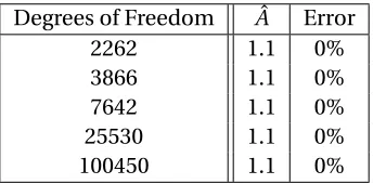
Table 3.2 Mesh refinement. A mesh refinement study showed that a finer mesh is un-necessary to maintain optimal accuracy of the hyperelastic model in a simple 1 mm by 1 mm square. . . 45
Table 3.3 Linear elastic versus hyperelastic convergence. A comparison between the lin-ear elastic and hyperelastic model shows that the linlin-ear model fails to converge above 30% strain. As expected outside the range of infinitesimal strains, the linear model will have issues converging. The hyperelastic model continues to work through all growth strains tested which supports our modeling choice of using a hyperelastic formulation rather than a linear elastic formulation for our simulations. . . 46
Table 4.1 Left-right (LR) endoderm and mesoderm width ratios in developing mice and frogs as calculated from the reported medians. The width the endoderm and mesoderm on the left and right side of the mouse and frog stomach changes as the stomach develops. Both sides begin with statistically the same size endo-derm, however the ratio of the left to the right decreases to become statistically significantly different from 1 over time as calculated by the authors of[Dav17]. This data was captured from plots in Figure 2E, F, M, and N in[Dav17]. Asterisks indicate values found to be statistically different from 1 as calculated by the authors of[Dav17]. . . 55
LIST OF FIGURES
Figure 1.1 Example of growth with material isotropy. For an isotropic material, isotropic growth results in dilation but no shape change. Where the same area change is maintained in this example, anisotropic growth here is shown as growth horizontally but not vertically. . . 6 Figure 1.2 Example of isotropic growth with material anisotropy. For an anisotropic
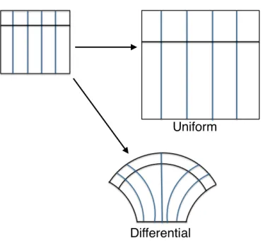
ma-terial, isotropic growth can result in shape changes. In this case the material is stiffer vertically than horizontally and when grown isotropically does not extend as much in the vertical direction. When material properties are the same in every direction and the domain is grown isotropically, the shape enlarges. . . 7 Figure 1.3 Uniform growth compared to differential growth. Uniform, isotropic growth
of an isotropic material results in a dilation of the original shape and is an affine transformation. Differential growth in an isotropic material results in a change of shape and may not be an affine transformation. . . 8 Figure 1.4 Types of growth for isotropic materials, illustrated on a cylinder. Isotropic
uniform growth is an enlargement of the original body. Uniform anisotropic growth is shown for each of the cylindrical coordinate directions(r,θ,z)with stretch ratiosλr,λθ, andλz. Inhomogeneous isotropic growth, where the growth is different in certain areas of the domain, causes obvious shape change. We consider this geometry further in Chapter 2. . . 9 Figure 1.5 Mapping of the initial configuration to the deformed configuration.B0is the
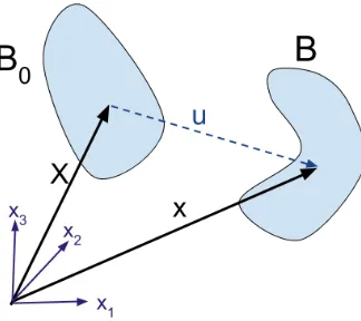
initial configuration with position vectorX.Bis the deformed configuration with position vectorx. The initial position vectorX can be mapped to the deformed configuration’s position vectorx using the displacement vectoru. 10 Figure 1.6 Application of growth and elastic tensors to an initial configuration. Only
considering the growth tensorGcan lead to incompatibilities in the body. Coupled with an elastic deformation tensorAhowever, these incompatibili-ties are resolved. Both the growth tensor and the elastic deformation tensor in this order under right polar decomposition give the overall deformation tensorF. Image adapted from[Rod94]. . . 12
Figure 2.2 Growth of a cylinder. For a cylinder of radius 1 mm and height of 2 mm, we set diag(G)=(1,1,2) in order to double the height. We had no stress boundary conditions on all the faces, no external pressure, and no displacement or rotation at an arbitrary point. To reflect our models in later chapters, we also chose to have noz displacement at on the bottom face of the cylinder. The error between our analytical volume and the calculated deformed volume ˆV was 0.0002%. . . 30 Figure 2.3 Depiction of shell element. The n direction is locally normal to the shell
midsurface, and theαandβ directions follow the directions of principal curvature, after[Smi05]. . . 33
Figure 3.1 Domain and boundary conditions used to solve for local coordinate systems in an example 2D domain. We solve∇2q =0 in the domainΩ. There are no flux boundary conditions,n· ∇q =0, on∂Ω1and∂Ω3. Without loss of generality at∂Ω4q=1 and at∂Ω2q=0. . . 40 Figure 3.2 Curves following the direction of the gradient ofqfor calculating local
coor-dinates. We calculated the curves of an example vector field from the Laplace equation with an inletq=1 on the bottom right face and an outletq=0 on the bottom left face. Notice how the calculated curves follow the curve of the domain. . . 41 Figure 3.3 Local curvilinear coordinate system. Our local curvilinear coordinate system
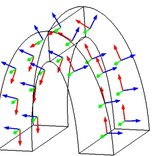
was calculated in this example for half of our stomach geometry seen later in Chapter 4. The first basis vector, in red, follows the curves of the domain, the second basis vector, in green, is in thez direction, and the third, in blue, is locally orthogonal to both the previous vectors. . . 41 Figure 3.4 Example domain with a clear analytical solution. We tested the accuracy of
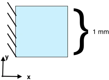
our model in a simple 1 mm by 1 mm square whose new dimensions we would be able to calculate analytically. This two-dimensional geometry was used for many tests to compare the hyperelastic model to the linear elastic model and check the accuracy of each. . . 44 Figure 3.5 Doubling the width and halving the height of a square. Even with strains as
large as 100%, the multiplicatively decomposed hyperelastic model remains accurate. Here we implemented a 100% strain in thex-direction and a -50% strain in they-direction to create a 2 mm by 1 mm rectangle from our 1 mm by 1 mm square. Area is conserved. . . 47
Figure 4.2 Simplified 2D histology. The simplified histology for the our model incor-porates the four distinct sections of the stomach (right and left endoderm and right and left mesoderm) and the liver, for completeness, with colors corresponding to the previous figure. The size of the stomach at this stage is approximately 400µm by 200µm, based on measurements from[Dav17]. Note that the right side of all images corresponds to the left side of the stomach as in[Dav17]from an anterior viewpoint. All directions are stated in reference to this orientation. . . 50 Figure 4.3 Test of stiffness effects. (A) has the maximal stiffness ofE =1000 Pa on the
interior and the minimal stiffness ofE =100 Pa on the exterior. (B) is meant as a control where both domains have the same stiffnessE =100 Pa. (C) has the maximal stiffness ofE =1000 Pa on the exterior and the minimal stiffness ofE =100 Pa on the interior. In the simulations shown, areas of positive stress (tension) are depicted in blue and negative stress (compression) are depicted in red. . . 52 Figure 4.4 Tests for growth location. Each column represents a different scenario of
domain expansion. As the endoderm expanded in (A) it began to curve the opposite direction of what was anticipated. (B) Both regions expanded and it curved in the correct direction. However (C) had the most dramatic curve. In the simulations shown, areas of tension are depicted in blue and compression are depicted in red. . . 53 Figure 4.5 Growth in the domain as compared to the boundary. The columns compare
(A) expanding the left side mesoderm to (B) growing the left side’s boundary. The left boundary expansion did not give the expected qualitative result. In the simulations shown, areas of tension are depicted in blue and compression are depicted in red. . . 54 Figure 4.6 Parametric study of isotropic stretch ratio as it affects curvature. A
represen-tative sample from our parametric study shows growth strains of (A)λ=1, (B) 1.25, and (C)1.5 in the mesoderm layer. More dramatic curvature is seen at the higher values ofλ, as predicted. In the simulations shown, areas of tension are depicted in blue and compression are depicted in red. . . 54 Figure 4.7 Size comparison of endoderm to mesoderm. At Stage 34 and 39, the endoderm
is the larger tissue on the left and right sides of the frog stomach. The change of left and right endoderm size over time is quantified in Table 4.1. From [Dav17]. . . 56 Figure 4.8 Simplified 3D geometry for the undeformed stomach. For all subfigure
Figure 4.9 Boundary conditions for the half domain. Due to the initial symmetry of our domain, we computed our model on a half domain. The bottom two faces have a symmetry boundary condition, meaning they have no normal displacement to the cut plane. We pinned a point, giving it no rotation and no displacement. All other surfaces have a no stress boundary condition, ˆnσ=0. As an additional modeling assumption due to surrounding tissues, the two posterior faces cannot move normal to the plane but are free in the other directions. . . 57 Figure 4.10 Local coordinate system(R,h,z). The black arrows give the local coordinate
directions from the origin. The green vector arrows represent the axial direc-tionz. The red vector arrows represent the hoop directionh and the blue vector arrows represent the radial directionR. . . 58 Figure 4.11 Isotropic growth of the left side of the stomach and no growth of the right
side. The stretch ratio in each direction isλR =λh=λz =1.2. Under isotropic growth, the geometry becomes asymmetric and very slight bending relative to the applied growth is seen in the biologically anticipated direction in (A)-(C). This bend may increase given a higher stretch ratio. (C) The cut view is shown in perspective to aid with visualization of the bending. . . 61 Figure 4.12 Anisotropic growth on the left side in the radial direction. The stretch ratios
areλR =1.2,λh =1,λz =1. We observe thickening in the left side of the stomach in (A) and no bending in (A)-(C). Neither outcome is consistent with the shape changes seen in the developing frog stomach. . . 61 Figure 4.13 Anisotropic growth on the left side in the hoop direction. The stretch ratios are
λR =1,λh=1.2,λz =1. The stomach appeared to extend in the dorsal-ventral direction in (A) but does not bend in the biologically anticipated direction in (B)-(C).This is not consistent with the shape changes seen in the developing frog. . . 62 Figure 4.14 Anisotropic growth on the left side in the axial direction. The stretch ratios are
λR =1,λh=1,λz =1.2. In (A)-(C), the deformed geometry shows bending from the left side over to the right side. However, it fails to show the radial thinning observed in[Dav17]. . . 63 Figure 4.15 Volume conserving anisotropic growth on the left side in the radial direction
with shrinking in the axial direction. The stretch ratios areλR =1.2,λh = 1,λz =1/1.2. This shows the deformed right side crossing over into the left in (A)-(C) which is not consistent with what is seen in the embryonic frog. . . 64 Figure 4.16 Volume conserving anisotropic growth on the left side in the radial direction
Figure 4.17 Volume conserving anisotropic growth on the left side in the radial direction with shrinking in the axial direction and contracting in the hoop direction. The stretch ratios areλR=1.2,λh=1/
p
1.2,λz=1/
p
1.2. In all views (A)-(C), the deformed right side crossed over into the left which is not consistent with what is seen in the embryonic frog. . . 65 Figure 4.18 Volume conserving anisotropic growth in the hoop direction with shrinking
in the axial direction. The stretch ratios areλR=1,λh=1.2,λz =1/1.2. (B) and (C) show bending in the opposite direction seen in[Dav17]. . . 66 Figure 4.19 Volume conserving anisotropic growth in the hoop direction with shrinking
in the radial direction. The stretch ratios areλR =1/1.2,λh=1.2,λz =1.(A) This shows bending in the opposite direction seen in[Dav17]though not to the extreme of the previous Figure 4.18. . . 66 Figure 4.20 Volume conserving anisotropic growth in the hoop direction with shrinking
in the radial and axial direction. The stretch ratios areλR =1/
p
1.2,λh = 1.2,λz=1/
p
1.2. (B)-(C) Bending is in the opposite direction seen in[Dav17]. 67 Figure 4.21 Volume conserving anisotropic growth in the axial direction with contraction
in the hoop direction. The stretch ratios areλR=1.2,λh=1/1.2,λz = 1.2.(B)-(C) show bending in the biologically anticipated direction. . . 68 Figure 4.22 Volume conserving anisotropic growth in the axial direction with thinning in
the radial direction. The stretch ratios areλR=1/1.2,λh=1,λz =1.2. ( A)-(C) show bending in the biologically anticipated direction and (A) includes the thinner width on the left seen in[Dav17]as well. . . 68 Figure 4.23 Volume conserving anisotropic growth in the axial direction with
contrac-tion in the hoop direccontrac-tion and thinning in the radial direccontrac-tion. The stretch ratios areλR =1/
p
1.2,λh=1/
p
1.2,λz=1.2. (A)-(C) all show bending in the biologically anticipated direction . . . 69
Figure 5.1 Three modes of lung branching as defined and shown in[Met08]. The three modes of lung branching were defined as domain, planar, and orthogonal branching. For domain branching, new lung bud tips grow from the sides of an existing stalk. For planar bifurcation, the tip of an existing lung bud splits and this pattern continues iteratively. This results in lung tips that all lie on a line, as seen in the end view of the figure. For orthogonal bifurcation, the tip of a lung bud splits but the next generation of splitting is rotated 90o. This results in lung bud tips that do not exist along the same line but rather in a plane, as seen in the end view of the figure.[Met08]hypothesized that these different modes were all caused by different mechanisms. Reproduced from [Met08]. . . 73 Figure 5.2 Packing of lung buds.Adisplays the an example partitioning of a mouse lung
Figure 5.3 Simplified histology of a single lung branch tip. Our simplified histology for a single lung branch tip includes the mesothelial surface, mesenchyme, epithelium, and lumen. The epithelium is a thin barrier tissue separating the mesenchyme from the lumen. Morphogens diffuse from the signaling mesothelial surface, represented by the blue line, through the mesenchyme, to be absorbed or bound on the epithelium, represented by the solid black line. Morphogen flux to the epithelium drives the shape change of the epithelium. 78 Figure 5.4 Geometric measures in an E12.5 mouse lung annotated from[Jon19]left
and [Mai01]right. 2RM is the full distance from one epithelial surface to another. We consider half this distance to be the location of the edge of our mesenchyme in our region of interest, where our region of interest can be considered to be the zone inside the blue dashed line.Φis the thickness of the epithelium, assumed to be constant.Lis the distance between the basal epithelial surface and the pleural surface through the mesenchyme.Re is the distance across the lung bud from basal epithelial surface to basal epithelial surface. . . 79 Figure 5.5 Domain and boundaries for the transport model. InΩ,D∇2c =0. The
bound-ary condition for the pleural surface,∂ΩP, is ˆn·D∇c =k, meaning the mor-phogen is being produced at a constant rate represented as a constant flux. The boundary condition for the sides∂ΩS and bottom∂ΩB is ˆn·D∇c =0, because our region of interest has no net flux given that it is modeled as pack-ing with its neighbors. The boundary condition for the epithelium,∂ΩE, is given byc=0, meaning all morphogen is assumed to be absorbed there. . . . 80 Figure 5.6 Local orthogonal coordinates for the shell. The local coordinates(η1,η2,η3)
have corresponding unit vectors that are tangential in the direction of maxi-mum curvature, tangential in the direction of minimaxi-mum curvature, and nor-mal to the shell surface, respectively. A representative shell piece is shown with its local coordinate system. . . 82 Figure 5.7 Location in shell. The bottom or apical surface is considered to be located
at ˜z =−1 and the top or basal at ˜z =1. In this two dimensional figure, the midsurface is represented by a dotted line. In thin shells planes normal to the midsurface, with the normal direction represented by the blue arrow in this two-dimensional simplification, remain normal to the midsurface even after deformation. In thick shells, that is not necessarily the case. For our model, we consider the positive normal direction to be oriented away from the lumen towards the mesothelial surface, or apicobasally. . . 85 Figure 5.8 Sketch of lung ROI geometry. (A) The cross section view shows a dotted line
Figure 5.9 Boundary condition on cut plane. For a top down view, withΦdisplaying the thickness of the shell, we have a plane of symmetry in red. All surfaces of the shell are under no stress, the surfaces touching the cut plane cannot move normal to the plane or rotate, and bottom surface of the plane also has no normal displacement. . . 87 Figure 5.10 Local ROI geometry of a cylindrical epithelium tubule nested in a larger
cylindrical mesenchyme and its morphogen flux distribution pattern. AsL decreases, the circular morphogen flux hot spot becomes a morphogen flux ring, denoted by "O". The authors of [GL18]hypothesized that a circular morphogen flux distribution pattern would correspond to tubule extension, while an annular morphogen flux distribution pattern was hypothesized to result in the the tip of the tubule dimpling or flattening. As annotated from [GL18]. . . 88 Figure 5.11 Flux and growth of epithelium of circular cross section inside a mesenchyme
of circular cross section. As previously defined,L is the distance between the basal epithelial surface and the pleural surface inµm. In the local cross-sectional geometry of an epithelium of circular cross section nested in a mesenchyme of circular cross section with a cross-sectional area ratio of 1:4, we considered severalLvalues. Higher normal flux magnitude is displayed in darker colors. Larger values forLlead to a circular flux distribution pattern and epithelial extension towards the pleural surface, while small values ofL lead to an annular region of higher flux magnitude and epithelial extension but no perceptible flattening. . . 89 Figure 5.12 Epithelium of circular cross section inside a mesenchyme ROI of elliptical
cross section. Large values ofLresult in circular hot spots, while a smallL value shows a split in the area of high flux distribution. In[GL18], the authors hypothesized that single hot spots for this geometry would cause extension of the epithelium, while tip splitting or branching of the epithelium is hy-pothesized to occur for split hot spots when an epithelium of circular cross section is inside a mesenchyme of elliptical cross section. Image annotated from[GL18]. . . 90 Figure 5.13 Flux and growth of epithelium of circular cross section inside a mesenchyme
Figure 5.14 Epithelium of elliptical cross section in a mesenchyme circular cross section. The flux distribution splits into two hot spots asLdecreases. In[GL18], tip splitting or branching is hypothesized to occur for split flux distributions, like that seen whenLis small in a local geometry of an epithelium of elliptical cross section is inside a mesenchyme of circular cross section. LargerLvalues for this geometry cause a single hot spot. This hotspot is hypothesized to lead to epithelial extension towards the pleural surface. Image annotated from [GL18], . . . 92 Figure 5.15 Flux and growth of epithelium of elliptical cross section inside a mesenchyme
of circular cross section. In the specific region of interest of an epithelium of elliptical cross section inside a mesenchyme of circular cross section with cross-sectional area ratio of 1:4, we considered L = 10, 20, 30µm. Darker colors correspond to higher local values of normal flux magnitude. Single morphogen flux hot spots, corresponding to higherLvalues, showed consid-erable extension towards the pleural surface. . . 93 Figure 5.16 Flux distribution of an epithelium of elliptical cross section inside a
mes-enchyme of elliptical cross section. In[GL18], single morphogen flux hot spots, seen for the larger L values, for this geometry are hypothesized to lead to epithelial extension towards the pleural surface, while tip splitting or branching of the epithelium is hypothesized to occur for split morphogen flux hot spots, seen for smallerLvalues, when an epithelium of elliptical cross section is inside a mesenchyme of elliptical cross section. Image annotated from[GL18]. . . 94 Figure 5.17 Flux and growth of epithelium of elliptical cross section inside a mesenchyme
of elliptical cross section. Our flux distribution matches that seen in[GL18]. Extension of the tubule is seen with single morphogen flux hot spots, seen for the largeLvalues, and some shouldering occurs with all values. . . 95 Figure 5.18 Differences in shape change caused by varying epithelial thickness.
Compar-ing the thickness of the epithelium fromΦ=15µm toΦ=5µm, we observed that epithelial thickness caused variation in shape change due to growth. No-tice that as seen from the top forΦ=5µm the shell changed its cross-sectional aspect ratio much more significantly than forΦ=15µm. . . 97 Figure 5.19 Self intersection due to epithelial thickness and interaction with overall shape.
For an epithelial cross section with minor axis 20µm and major axis 40µm and thickness ofΦ=15µm, simulations converge but the shell self-intersects. This is not biologically realistic. . . 98
Figure A.2 Application of local growth strain to a solid cylinder in a cylindrical coordinate system. Using a cylinder that has a height to radius ratio of 3:1, we tested the solid mechanics version of this problem. Going from left to right, we increased the strain by 5% increments from 5% to 20%. More dramatic shape changes would be expected at 20% than at 5%. The color bar represents first principal strain. In (A)-(B), we tested cell rearrangement cases. In (A), the cylinder grew circumferentially but the height shrank and in (B) its height grew but it decreased circumferentially. (C)-(E) are the cellular division cases, where volume is not conserved. In (C) the cylinder grew circumferentially, in (D) along the height, and in (E) in both directions. . . 112 Figure A.3 Application of local growth strain to a cylindrical shell in a cylindrical
co-ordinate system. Using the shell formulation instead, we tested the same geometry and growth models as in Figure A.2. Going across we increased the strain from 5% to 10% to 20%. 15% was disregarded because it gave no addi-tional information. The color bar represents first principal strain. In (A)-(B), we tested cell rearrangement cases. In (A), the cylinder grew circumferentially but the height shrank and in (B) its height grew but it decreased circumferen-tially. (C)-(E) are the cellular division cases, where volume is not conserved. In (C) the cylinder grew circumferentially, in (D) along the height, and in (E) in both directions. . . 113 Figure A.4 Effects of boundary conditions. To emphasize that boundary conditions can
drastically affect results, two similar cases are shown. Going across the strain is increased by 5% from (A) 5%, (B) 10%, (C) 15%, and (D) 20%. The color bar represents first principal strain. The top row is where this shell formulation has no vertical displacement only on the bottom of the cylinder. The bottom row is where it has no vertical displacement on both the top and bottom of the cylinder. All other conditions are exactly the same. Notice that the top row has interesting dimpling or buckling above the area of strain. . . 114 Figure A.5 Cylindrical shell strained while surrounding a solid material. Using the shell
formulation but with a relatively low stiffness solid inside, we tested the same geometry. Going across we increased the strain from 5% to 10% to 20%. From top to bottom, we grouped cell rearrangement together, first increasing height and then increasing circumferentially. Then we grouped volumetric growth together increasing in height, then circumference, and then both. Notice that there is very little overall deformation and the strained circle remains in a very similar location and configuration compared to how it began. The color bar represents first principal strain. . . 115
Figure B.2 For the same element, the left square shows the interpolation points for the displacement,u, and the rotation,θas black circles. The additional purple circle represents an additional interpolation point for the rotation only. In the right square, the tying points are represented by crosses and labelled A through H. As represented in the local coordinates (r,s), A is at (1/p3, 1) and C is at (-1, 1/p3). Notation after that in[CB11]. . . 117 Figure B.3 Locking of numerical methods. As shown for a linear elastic solid
CHAPTER
1
OVERVIEW
The termmorphogenesisdescribes the processes of growth, cell division, reorganization, and
restructuring of a tissue, organ, or organism that change its morphology. We used the emerging field
ofmorphoelasticityto model morphogenesis in two complex biological systems, specifically lung
branching and stomach bending. Many popular extant morphogenetic models such as agent-based
models are not grounded in a physics framework though can be informative when formulated
correctly. Using the mathematical theory of morphoelasticity allows us to model complicated
systems while still considering the underlying physics.
The stomach in many species has a distinctive curved shape which is important for the proper
function of the organ. This curve creates left-right asymmetry in the stomach. We will evaluate
hypotheses on the cause of stomach bending due to varying left-right levels of: (a) mitosis, (b) cell
rearrangement, or (c) a combination. Models (b) and (c) are mathematically novel in that they
thesis, we ruled out that a greater rate of overall mitotic growth on the left side of the stomach as
compared to the right is cause for the asymmetric bending in the stomach. Instead, we concluded
that anisotropic growth, representing different oriented cell rearrangements or divisions on the left
and right sides of the stomach, is necessary to obtain the shape changes seen in the developing
stomach.
Lungs begin as a single tube that then goes through many iterations of branching in many
directions to become fully formed. We will determine the pseudoglandular lung shape changes
resulting from growth governed by different morphogen flux distributions as asserted in[GL18].
Our lung models will be the first lung models to include the framework of morphoelasticity, and
one of the first morphoelastic models to incorporate thick shell theory. For our novel application,
we explicitly modeled both the morphogen signaling, which depends strongly on local geometry,
and the resulting growth dependent on the calculated morphogen flux distribution. Unlike many
previous models of lung branch growth, we also considered the differences that epithelial thickness
may yield in the final shape. Anticipated outcomes from these models will either support or refute
proposed biological hypotheses.
1.1
Organ Morphogenesis
Mathematical aspects of morphogenesis have been described as early as 1917 by D’Arcy Thompson
[Tho61]. Morphogenesis can occur in both developing organisms and in mature organisms, such as
during lactation or the formation of tumors. In early development, organs can rapidly change in size,
shape, and even material properties. Specifically in early development,organogenesisis the term
used for the process where the ectoderm, mesoderm, and endoderm form the internal organs. These
tissues further differentiate during development. We specifically focus in this thesis on two kinds of
tissues: epithelium and mesenchyme. Anepitheliumis a sheet-like tissue that lines the surfaces
of organs and separates tissues from each other and from the lumen, a fluid-filled cavity. The size
and shape of epithelial cells depend on their function and location but in general they are tightly
a lumen; thebasalsurface of an epithelium is in contact with another tissue. Our second tissue of
interest is themesenchyme. The mesenchyme is a tissue containing some widely separated cells in
an extracellular matrix (ECM). Often considered connective tissue, the mesenchyme fills the space
between epithelia.
To aid in clarity when discussing morphogenesis and early development in general, humans
are classified by 23 Carnegie stages which are divided roughly by size, timing, and morphological
characteristics[OM01]. These stages have been adapted to other animals and allow us to compare
timing during development between species. For mice, it is common practice to refer to embryonic
days since timed pregnancy as E and then the day, for example E12.5, and further development
after birth begins with P for postnatal. For example, Carnegie stage 16, which is in humans at day 40,
in mice is at E12.5. It is important to note that these stages are of varying time periods in humans,
between one day and nearly one week. This time period discrepancy arises because the the stages
are divided based on morphological events, such as limb bud formation or notochord detectability,
which do not occur uniformly over time.
1.1.1 Stomach Organogenesis
The embryonic stomach in many vertebrates begins as a straight tube which undergoes significant
shape change to become an asymmetric, multiply curved, bent, elliptical tube. This left-right (LR)
asymmetry is seen in many organs throughout the body. "Left-right (LR) asymmetry is a fundamental
feature of internal anatomy, yet the emergence of morphological asymmetry remains one of the
least understood phases of organogenesis. Asymmetric rotation of the intestine is directed by forces
outside the gut, but the morphogenetic events that generate anatomical asymmetry in other regions
of the digestive tract remain unknown"[Dav17]. We consider the change in stomach shape in
Xenopus laevisfrog embryos from the commonly defined developmental stages 34-39. At stage 34
the embryonic frog stomach is symmetrical, but as it grows, significant asymmetry emerges. In both
mice and frogs, the asymmetry of the stomach is known to depend on left-right patterning genes,
1.1.2 Lung Organogenesis
The mature lungs are a richly branched organ that exhibits fractal-like space filling. This results in
the large gas exchange surface area essential to the proper function of the lung. Its mature shape is
produced by a variety of mechanisms throughout development. In mice, lung organogenesis begins
at E9.5 and goes through four major fetal stages[Mas04]. The first is the pseudoglandular stage
where branches are formed occurring between E12 and E16.5. Then there are two intermediate
stages, the canalicular and saccular, occurring between E16.5 and P4. Further structural changes
occur during the alveolar stage from the post-natal development stages P4-P14. We consider the
branching of embryonic lungs in the pseudoglandular stage. Epithelium-mesenchyme interaction
in branching is essential; experiments have shown that “after removal of the mesenchyme at the
growing tip, further branching of the epithelial tubules is prevented"[Mas04]. The morphogenetic
behavior of the epithelium has been linked to a number of genes and growth factors such fibroblast
growth factor 10 (FGF10), transforming growth factor beta (TGF-β), and sonic hedgehog (Shh)
among others. While many chemicals have been associated with branching, the exact mechanisms
that cause specific branching patterns and the mechanics behind this are a continuing area of
research.
1.2
Morphogenesis Modeling Overview
Morphogenesis is the process by which growth and cell rearrangements alter the shape of a
devel-oping tissue. Shape change can be described mathematically as a rearrangement of the relative
positions of material points in the body. Many different approaches have been taken to model
morphogenesis. We can subdivide the main approaches into continuum-based or agent-based.
Common continuum models are based in the theories of poroelasticity, fluid dynamics, solid
me-chanics, mixture modeling, or are just phenomenological. Agent-based model approaches include
1.2.1 Agent-based Modeling Approaches
Agent-based modeling approaches focus on describing individual cell interactions. Agent-based
computational models use individual agents that interact following set rules, and can be
deter-ministic or stochastic. One agent-based approach to morphogenesis, vertex modeling, models
individual cells as polyhedra where multicellular interactions are defined by vertex movements
[Hon04]. Vertex models have been used to simulate tissue morphogenesis but do not include a full
physics framework[Oku14],[MI08] [Bar17]. Cellular Potts models, which are stochastic, consider
the adhesion between cells to be a driving factor for deformation[Mer06],[SM13],[Hes11]. Using
the definition in[GG92], in cellular Potts models a cell’s location is defined by a number of adjacent
lattice sites. The set of lattice coordinates that defines the cell changes as the cells move and grow as
determined by a minimization process of a pseudo-energy function. Hybrid cellular Potts models
consider cell movements discretely but model chemical signaling in a continuum[Oer14].
1.2.2 Continuum Modeling Approaches
In continuum modeling, one considers objects to be completely space-filling rather than discrete
particles and considers changes to be occurring in some neighborhood around any particular point.
For continuum based approaches, a general theory for soft, elastic tissues with finite volumetric
growth that mathematically described the relation between stress and growth was developed in
[Rod94]. For hard tissues like bone, it has been well established that stress and strain can modulate
growth[Rod94]. However, soft tissues, unlike hard tissues, can experience large elastic deformations
and become residually stressed[Rod94]. Stress is not only a potential result of growth but may also
affect the further growth of the body. Growth may introduce incompatibilities in the body, like
self-intersection, that can be resolved with the introduction of an elastic stress. The morphoelastic
framework developed in[Rod94]considers that the shape change during growth occurs as a result of
material being either added or removed, an elastic deformation, or both. The morphoelastic model
1.3
Isotropy, Anisotropy, and Inhomogeneity of Growth
For our morphogenesis problems, we consider the change in shape of individual organs. For the
purposes of this thesis, we hereafter consider "growth" to be a general term describing a shape
change and not necessarily an indicator of an increase in volume. Both growth and materials can
be considered isotropic or anisotropic. Shape change can be due to anisotropic growth, isotropic
growth of an anisotropic material, or inhomogeneous growth. Since they are all biologically different,
we will discuss the distinctions. For simplicity, we consider all materials in this thesis to be isotropic.
During morphogenesis, organs can experience growth, in potentially both volume and shape, as
cells divide, apoptose, and rearrange. Uniform isotropic growth of an isotropic material gives no
change in shape. Biologically that would be equivalent to mitosis, where the rate of mitosis was
uniform in every direction and at every location. Volume conserving anisotropic growth is a result
of cell rearrangements. Assuming isotropic material properties, Figure 1.1 illustrates the difference
between isotropic growth (growth equal in every direction) and anisotropic growth (growth that is
different in different directions) for a square whose area is quadrupling. If a material is anisotropic
then the material properties are not the same in every direction. Figure 1.2 illustrates an example of
isotropic growth in an anisotropic material.
Figure 1.2Example of isotropic growth with material anisotropy. For an anisotropic material, isotropic growth can result in shape changes. In this case the material is stiffer vertically than horizontally and when grown isotropically does not extend as much in the vertical direction. When material properties are the same in every direction and the domain is grown isotropically, the shape enlarges.
It is also important to consider differential growth, where the rates of volumetric growth are
different in different locations. Figure 1.3 shows an example of the difference between uniform
isotropic growth and differential growth.
Figure 1.4 summarizes several of these different types of growth on a cylinder where material
properties are assumed to be isotropic. Uniform isotropic growth results in a dilation of the original
cylinder. Uniform anisotropic growth results in a change of aspect ratio of the cylinder.
Inhomo-geneous isotropic growth results in a shape change and does not result in a cylinder. We consider
this geometry and the multiple types of growth further in Chapter 4. Notice that because we are
considering a cylinder in Figure 1.4 we are using the cylindrical coordinate system. Alternative
Figure 1.3Uniform growth compared to differential growth. Uniform, isotropic growth of an isotropic material results in a dilation of the original shape and is an affine transformation. Differential growth in an isotropic material results in a change of shape and may not be an affine transformation.
1.4
Mathematical Background
1.4.1 Morphoelasticity
Following the framework developed in[Rod94]and described in detail in[Gor17], we will explain the
morphoelastic model structure. In order to describe how a body undergoes a shape or volume change,
we consider its initial configuration,B0, and its deformed configuration,B. The relationship between a position vector in the initial configuration and a position vector in the deformed configuration
can represented by
x1=X1+u1, (1.1)
x2=X2+u2, (1.2)
x3=X3+u3, (1.3)
Figure 1.4Types of growth for isotropic materials, illustrated on a cylinder. Isotropic uniform growth is an enlargement of the original body. Uniform anisotropic growth is shown for each of the cylindrical coordinate directions(r,θ,z)with stretch ratiosλr,λθ, andλz. Inhomogeneous isotropic growth, where
the growth is different in certain areas of the domain, causes obvious shape change. We consider this geometry further in Chapter 2.
deformed bodies and their position and displacement vectors.
Formulating this as a mapping from the initial to the deformed configuration, the chain rule
yields
d xi= ∂xi
∂xjd Xj, (1.4)
Figure 1.5Mapping of the initial configuration to the deformed configuration.B0is the initial
configura-tion with posiconfigura-tion vectorX.Bis the deformed configuration with position vectorx. The initial position vectorXcan be mapped to the deformed configuration’s position vectorx using the displacement vector
u.
More generally, we could consider the mapping to be
Fi j= ∂xi ∂Xj
, (1.5)
whereFis a second-order tensor called thedeformation gradient tensorthat can be represented as
F=
∂x1
∂X1
∂x1
∂X2
∂x1
∂X3
∂x2
∂X1
∂x2
∂X2
∂x2
∂X3
∂x3
∂X1
∂x3
∂X2
∂x3
∂X3
. (1.6)
Differentiating each of the above terms with respect tox1,x2,x3yields the nine equations
∂x1 ∂X1
=∂X1 ∂X1
+∂u1 ∂X1
∂x1 ∂X2
=∂X1 ∂X2
+∂u1 ∂X2
∂x1 ∂X3
=∂X1 ∂X3
+∂u1 ∂X3
(1.7)
∂x2 ∂X1=
∂X2 ∂X1+
∂u2 ∂X1
∂x2 ∂X2=
∂X2 ∂X2+
∂u2 ∂X2
∂x2 ∂X3 =
∂X2 ∂X3+
∂u2
∂X3 (1.8)
∂x3 ∂X1
=∂X3 ∂X1
+∂u3 ∂X1
∂x3 ∂X2
=∂X3 ∂X2
+∂u3 ∂X2
∂x3 ∂X3
=∂X3 ∂X3
+∂u3 ∂X3
. (1.9)
gradient tensorFagain. Grouping the first terms on the right hand sides gives the Kronecker-delta matrix
δi j=
1 0 0
0 1 0
0 0 1
. (1.10)
The second terms from the right hand side of each of the nine equations are always the derivatives
of the displacement with respect to a coordinate direction, as shown
∂u1
∂X1
∂u1
∂X2
∂u1
∂X3
∂u2
∂X1
∂u2
∂X2
∂u2
∂X3
∂u3
∂X1
∂u3
∂X2
∂u3
∂X3
. (1.11)
Altogether, this yields the equation
∂x1
∂X1
∂x1
∂X2
∂x1
∂X3
∂x2
∂X1
∂x2
∂X2
∂x2
∂X3
∂x3
∂X1
∂x3
∂X2
∂x3
∂X3
=
1 0 0
0 1 0
0 0 1
+
∂u1
∂X1
∂u1
∂X2
∂u1
∂X3
∂u2
∂X1
∂u2
∂X2
∂u2
∂X3
∂u3
∂X1
∂u3
∂X2
∂u3
∂X3
. (1.12)
Therefore the deformation gradient tensor can be concisely represented as
Fi j=δi j+ ∂ui ∂Xj
, (1.13)
or, in more compact notation, as
F=I+∇u. (1.14)
This means thatFdescribes the local, relative deformations of an object using the spatial derivative of the mapping from the undeformed basis to the deformed basis. In order to generalize, if we
denote the deformation mapping byχand the define new bases{e1,e2,e3}and{E1,E2,E3}then
F=∇χ= ∂
∂xj(
In morphoelasticity, when a volume element of the initial unstressed configurationB0grows the size and orientation of the new volume element are described by thegrowth deformation tensorG. This growth deformation tensor, when applied to the volume elements ofB0, transforms the initial configuration to a virtual unstressed stateV. This virtual deformation, while unstressed, could result in incompatibilities in the continuum of the body. Figure 1.6 shows an example of such an
incompatibility. Incompatibilities include self-intersection and other topological changes that make
Figure 1.6Application of growth and elastic tensors to an initial configuration. Only considering the growth tensorGcan lead to incompatibilities in the body. Coupled with an elastic deformation tensor
Ahowever, these incompatibilities are resolved. Both the growth tensor and the elastic deformation tensor in this order under right polar decomposition give the overall deformation tensorF. Image adapted from [Rod94].
the unstressed deformed body an impossibility. However, introduction of anelastic deformation
tensorAresolves these.V, the virtual configuration, can be used to find both the elastic strains which ensure compatibility and the elastic stresses which ensure that the body loads are balanced
and the boundary conditions are met. These are defined by the elastic deformation tensorAwhich will mapV to the new configurationB. Taken together we can writeF=AG.
Further description of the structures ofF,A, andGcan be found using the polar decomposition theorem. The polar decomposition theorem, as used in[Rod94], states that: For a second-order
unique proper orthogonal tensorRsuch that
F=RU=VR. (1.16)
Note thatFis not necessarily non-singular, as det(F)≥0. The positive symmetric tensorsUandV are called theleftandright stretch tensors, respectively. Their squares can easily be obtained fromF as follows:
FTF=U2=C, the right Cauchy-Green tensor (1.17)
FFT=V2=B, the left Cauchy-Green tensor. (1.18)
SinceV=RURT(because orthogonal tensors’ inverses are their transposes),UandVhave the same eigenvalues. Because the eigenvalues ofUandVare the same, this means that given either of the Cauchy-Green tensors, finding the square root of eitherCorB’s eigenvalues is the same as finding the eigenvalues,λi of eitherUorV. Using the eigenvectorsui orviofUorVrespectively allows us to reformulateFanother way in three dimensions as
F= 3 X
i=1
λivi⊗ui. (1.19)
The polar decomposition theorem can also be utilized onGto guarantee that it can be sym-metrized. If we have anFthat is known thenAandGare not unique. We could, through the polar decomposition theorem, decomposeG, instead ofF, into
G=RGUG, (1.20)
where UG is a symmetric tensor andRG is an orthogonal tensor. In the morphoelastic models developed in this thesis, we will assume tissues are materially isotropic. In that case, the
be decomposed, we can state that
W(A) =W(FG−1), (1.21)
=W(FU−G1RTG), (1.22)
=W(FUG). (1.23)
Because the elastic energyW of an isotropic material depends just on the symmetric part of the growth tensorG, the deformation gradient tensorFcan be decomposed into an elastic deformation tensor and a symmetric growth tensor. This means that we will always considerGto be symmetric for an isotropic material. Specific choices for the formulation of the strain-energy density function
of a hyperelastic material will be described in detail in Section 1.4.3.
We can use the polar decomposition theorem in a different context to decouple growth from
rotation. As described in[Rod94],Gdecomposes into two pieces, thegrowth stretch tensorUgand therotation tensorRg. The growth stretch tensorUgcan be found by integrating the growth rate tensor over time, though in this thesis we do not grow bodies in time; rather, we consider a single
time step. Without loss of generality, the rotation tensorRgcan be considered the identity tensor because any rotation in the growth tensor can simply be incorporated into the elastic deformation
tensorAas shown by
F=AG, (1.24)
=ARgUg, (1.25)
=AUˆ g, (1.26)
where ˆAcan be considered new elastic deformation tensor andG≡Ug.
However,Gmerits a still closer look. The growth deformation tensorGdescribes how individual volume elements change their unstressed size, shape, and orientation. Note that if the determinant
configu-ration and the new configuconfigu-ration, but shape change could still have occurred. To describeGfor implementation in our models, we also needed to define a growth stretch ratioλ. This allows our
stretch ratios to be consideredλi j=1+εi j, whereεi j is the strain in thei jdirection. In Cartesian coordinates this allows us to writeGas
G=
λx x λx y λx z
λy x λy y λy z
λz x λz y λz z
. (1.27)
Further details can be found in Section 3.1.
Another essential tensor in our model framework is the Cauchy stress tensorT. The Cauchy stress tensorT=nσ, wherenis the normal vector andσis stress, describes stresses on a body and allows us to write the equation of motion
∇ ·T+ρb=ρv, (1.28)
whereρis the mass density, andv the velocity. In this thesis, we ignore any body forces sob is 0 and because we assume our tissue’s movement is only due to growth,v=0. Therefore the equation of motion for our models is
∇ ·T=0. (1.29)
The Cauchy stress tensorTis symmetric soT=TT. The Cauchy stress tensor and the elastic defor-mation tensorArelate through the strain-energy density functionW,
T=JA−1A∂W
∂A −p1, (1.30)
1.4.2 Continuum Mechanics
Mechanics and its interaction with gene signaling are essential to development and growth.
Specif-ically we consider thekinematicsof the growing body to be an important aspect. Kinematics as
defined by[Bla17]is the term for the geometric transformations that quantify morphogenetic change
without reference to force. We are especially focused on describing the stretch ratios of the growing
organs as defined by thestrain. While there are many mathematical formulations for strain, it can
be simply defined as the difference due to deformation of a domain relative to its original
configura-tion. Strain is a unitless measure.Stressis a description of the internal forces per area that occur
between neighboring particles in a material and its unit is commonly given as Pascals. In simple 1-D
cases, stress is linearly proportional to strain using a stiffness constant, usually Young’s modulus. To
properly formulate the nonlinear large-strain 3-D system of partial differential equations governing
the mechanics of growth, we must consider the morphoelasticity and hyperelasticity equations and
relate them to the standard continuity and balance equations with careful attention to the stresses
and strains from growth.
1.4.2.1 Solid Mechanics
Following our previously established theory from[Rod94]explained in Section 1.4.1, we also need to
include the framework of solid mechanics. We give the standard time dependent equations, however
for our modeling purposes we only consider the mechanics at steady state as will be further clarified
in Chapter 2. To begin, we consider the continuity equation
∂ ρ
∂t +∇ ·j=c−d, (1.31)
whereρis the mass density,j is the flux in the system,c is a source of mass, andd is a sink. We must consider changes in mass as the growing organs may experience unbalanced mitosis and
1.31 simplifies to
∇ ·(ρu) =0. (1.32)
We can also define the mass rate of growth as
˙
m=ρdivv, (1.33)
assuming that the mass densityρis constant and uniform everywhere Here,mis the mass andv is the growth velocity. The rate of unit tissue volume change is then described as
d V
d t =divv=tr(Dg), (1.34)
whereDg is the rate of growth tensor.Dg is then related to the growth stretch tensor by
Dg = 1 2(U˙gUg
−1+U
g−1U˙g). (1.35)
Recall that the growth stretch tensorUg is the non-rotational tensor fromG’s decomposition and without loss of generality this can be consideredGas shown previously in Equation 1.24, stating
F=AUˆ g. (1.36)
The deformation gradient tensor itself can be related to the deformation of the system given
F=I+∇u, (1.37)
whereIis the identity tensor and and∇uis the gradient of the displacement vector as previously expressed in Equation 1.14. The determinant ofF, representing the ratio between the current and initial volume, is written asJ =det(F). Recall thatFcan be multiplicatively decomposed into the elastic deformation tensorAand the growth deformation tensorG, orF=AG.
gradient tensorF=AGwith
0=∇ ·FS+FV, (1.38)
whereFV is the volume force vector andSis the second Piola-Kirchhoff stress tensor. The second Piola-Kirchhoff stress tensorSis symmetric and related to the Cauchy stress tensorTwhich was used previously by the equation
ST=JFF−1T. (1.39)
Sis sometimes referred to as the nominal stress and represents force over the original area, while Tis sometimes called the true stress and represents force over the deformed area. Consider the formulation of the deformation problems in terms ofS.Sis represented by
S=Sext+ ∂W
∂E, (1.40)
whereSextis any external stress which in this thesis is assumed to be 0,W is the strain-energy density function which on the hyperelastic model chosen, andEis the Green-Lagrange strain tensor. The Green-Lagrange strain tensor is given by
E=1 2(F
TF
−I). (1.41)
Because we assumed all materials to be incompressible and because material testing has shown
a linear stress-strain relationship in developing epithelia for moderately large stretch[Tab08], we
selected the neo-Hookean hyperelastic model. Hyperelasticity is further described in the following
section.
1.4.3 Hyperelasticity
As defined in[Fun65], non-Hookean nonlinear materials can be generalized into three basic types.
Elastic materialspossess a homogeneous stress-free natural state and in a finiteδ-neighborhood
the Almansi strain tensor. Often the Eulerian stress tensor is written directly as a function of the
deformation gradient tensorF, but this is only true for idealized materials. Materials are considered
hypoelasticif the components of the stress rate with respect to time are a homogeneous linear
function of the components of the rate of deformation and are not history dependent. We consider
hyperelasticmaterials for our models. Materials are said to be hyperelastic if there exists a
strain-energy density function where the rate of change of the strain-strain-energy density with respect to time is
equivalent to the rate of doing work using the stresses.
The objective of hyperelastic models is to describe the behavior of materials that do not satisfy
a linear relationship between stress and strain and they are especially useful when strains are not
infinitesimal. Given infinitesimal strains, many materials’ stress-strain relationships are
approxi-mately linear but soft tissues typically undergo large strains even without growth; so, we cannot
rely upon linear elastic theory as an accurate approximation. We use the notation and framework
as defined in[Hac18].The majority of widely used hyperelastic models relate to our morphoelastic
framework through the right Cauchy deformation tensorC. The principal invariantsI1,I2, andI3of the right Cauchy deformation tensor as defined in Equation 1.17 are used in many descriptions of
the strain-energy density function. They are defined in summation notation as
I1=trace(C) =Ci i, (1.42)
I2= 1 2
I12−Ci jCj i
, (1.43)
I3=det(C). (1.44)
1.4.3.1 Neo-Hookean
The simplest hyperelastic model is neo-Hookean. This model describes the strain-energy density
functionW as being
W =µ 2 I1−3
where µis the Lamé coefficient representing the shear modulus in continuum mechanics and
where 3µis the Young’s modulus. This model can be used for predicting the behavior of materials
undergoing large deformation whose stress-strain relationship is not necessarily linear. The
neo-Hookean model is a simplified form of the Mooney-Rivlin hyperelastic model. We chose to start
simply with a one parameter hyperelastic model in order to focus more on other aspects of the
problems.
1.4.3.2 Mooney-Rivlin
The Mooney-Rivlin hyperelastic model is well-defined in situations where the material is nearly
incompressible or when the bulk modulus of a material is a few orders of magnitude larger than the
shear modulus. This model is defines the strain-energy density function to be
W =C1 2 I1−3
+C2
2 I2−3
, (1.46)
where for small strains 2(C1+C2)is the shear modulusµand 6(C1+C2)is the Young’s modulus. With the bulk and shear moduli difficult to determine in soft, developing tissues, we decided against
using this model.
1.4.3.3 Fung
For strain-stiffening materials especially for soft biological materials like arteries, a Fung
hypere-lastic model is often used. There are many different formulations of Fung hyperehypere-lastic models; we
considered the one given in[Hac18]. In this case the strain-energy density function is considered to
be
W =c 2(e
Q
−1) +K 2
(JA)2−1 2 −lnJA
, (1.47)
parameters, we instead used the neo-Hookean hyperelastic model.
1.5
Summary of Morphoelastic Framework
Collecting the equations developed in this chapter together into an overarching framework we have
F=AG=∇χ deformation gradient tensor (1.48)
∆V
V =det(G) volume change equation (1.49)
divT=0 equation of motion (1.50)
T=TT =J−1F∂W
∂F −p1 constitutive law (1.51)
W =µ 2 I1−3
Neo-Hookean strain-energy density function. (1.52)
These equations, while not a complete list of every relation, are the most essential to our
morpho-genetic framework and will be referenced in later chapters. An alternative formulation with respect
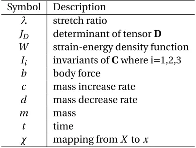
to the reference variables can be found in[Gor17]. The growth tensorGis an input to our system and will be defined differently for the two systems developed in Chapters 4 and 5.Gwill be explained in further detail in these chapters as their individual local coordinate systems are established. Tables
1.1-1.5 list all tensor, parameter, variable, and geometry names.
The rest of this dissertation is organized as follows. Chapter 2 establishes the details of the
solid and shell mechanics and gives the analytical solutions to a few examples. Chapter 3 describes
the implementation and verification of our model systems. In Chapter 4, we apply our modeling
framework to test different hypotheses on the causes of stomach bending using solid mechanics.
In Chapter 5, for different local regions of interest we solve a morphogen transport problem to
inform the growth of a lung tubule using shell mechanics to test hypotheses relating morphogen
flux distributions to epithelial shape changes. Chapter 6 contains a discussion of our results and