Division VIII, Paper ID 739
MONTE-CARLO BASED RELIABILITY/AVAILABILITY ANALYSIS
ALGORITHM FOR EFFICIENT MAINTENANCE PLANNING
Hindolo George-Williams
1, Edoardo Patelli
2 1Centre for Doctoral Training on Quantification and Management of Risk and Uncertainty in Complex Systems & Environments, Institute for Risk and Uncertainty, University of Liverpool, United Kingdom
2
Institute for Risk and Uncertainty, School of Engineering, University of Liverpool, United Kingdom
ABSTRACT
Failure is an effect inherent in all mechanical and electronic components either as a consequence of their operating conditions or a consequence of their age. This makes a system prone to failure at any point in its operating period; a measure of the likelihood of these failures is the reliability of the system. It is an important quantity that can be used to assess the performance of a system both quantitatively and qualitatively. Preventive & corrective maintenance can reduce the occurrence of failures in a system and their duration. Therefore, the performance of a multi component system depends on the quality of its preventive and corrective maintenance schemes.
This paper presents a generalised approach to analysing the reliability and performance of multi state component, multi output engineering systems using Monte Carlo simulation. With its ability to implement any failure/repair distribution, restrictive maintenance and specific switching procedures given the unavailability of a component or set of components, the algorithm can be used to analyse (without making the usual assumption of exponential failure/repair) the response of a multistate system to a series of maintenance policies. The approach also presents an efficient means of incorporating cost analysis in reliability and performance analysis.
The applicability of the approach is shown by the analysis of a 50MW, two-unit Hydroelectric Power Plant. The methodology is generally applicable and may be used to support the identification of a robust maintenance strategy for many engineering systems including Nuclear Power Plants.
INTRODUCTION
Many engineering systems consist of a complex interconnection of smaller components and subsystems; continuous operation of the system without failure or unwarranted interruptions is virtually impossible. The effect of these failures can range from a few hours of power cut in the electricity industry to reduction in profit margin due to lost time in the manufacturing industry. Therefore, it is important to be able to predict how often these failures occur and their potential effect on the system for enhanced decision making.
Reliability prediction has been a very important tool for reliability engineering since the 1950s (Saleh, Marais 2006). Since then, it has seen tremendous development moving from traditional methods that consider the failure of a system as being a consequence of only its components to methods that look at the failure of a system from a wider perspective including external factors (Denson, 1998).
Division VIII made are close enough to the actual operating conditions. Hence there are significant levels of uncertainties associated with this process depending on the methodology used.
In the last two decades various researchers have done significant work in this field, Majeed et al. (2006), Cristina et al. (2009) and Veeraraghavan et al. (1994) being a few examples. The analyses in these works were mainly based on the Markov Chain technique. One set back of Markov analysis is that it cannot model uncertainties such as restrictive maintenance schemes, human, environmental and other stochastic external factors which may affect the performance of a system. Real engineering systems are multi component in nature with components exhibiting different failure/repair characteristics and existing in one of more than two states at any instance. Markov Analysis often assumes exponential or Weibull failure/repair, two-state behaviour of components, requires complicated mathematics and becomes complex with increase in size of the system. The number of states in the model in the model may be up to ʹ where m is the number of components making up the system. Therefore at large values of m the number of states increases dramatically which makes the model difficult to construct and expensive to compute (Reliability Analysis Center, 2003). Veeraraghavan et al. (1994) used a combinatorial algorithm that requires the introduction of a dummy component of ʹ states to implement shared repair (where m is the total number of components sharing the repair team) rendering the methodology cumbersome for realistic complex engineering systems. Analytical methods therefore cannot adequately evaluate the performance of realistic multi component engineering systems.
In this work, we propose a strategy and computational tool that addresses the inadequacies of existing methodologies. The approach can be applied to many system configurations with relative simplicity. It keeps track of the various activities (transitions) of the system and its building block as the simulation proceeds. These transition histories are used to evaluate the performance of the system both at the system and component levels.
Monte Carlo simulation was incorporated into the computational tool to enhance the modelling of stochastic events that would otherwise be impossible to model by analytical procedures like Markov Methods.
FEATURES AND ASSUMPTIONS USED
In the approach, the operation of the system is simulated based on the failure and repair data of the components making up the system, maintenance policy of interest and returns the reliability indices of the system.
Component Modelling
In practice, the performance of an Engineering system is influenced to a greater extent by external events which are normally stochastic in nature. External stochastic events such as availability of spares, administrative protocols and availability of maintenance personnel have the potential to prolong response to a fault. The algorithm models the effects of availability of spares, administrative protocols, maintenance personnel and maintainability of system components on system reliability and performance. To implement these stochastic events, each component of the system is modelled as a multi-state object as shown in Figure 1. The number of states may be less or more than what is depicted by Figure 1 depending on the system being analysed and the stochastic events considered. This allows the introduction of additional states for components with multiple failure modes and standby systems. For instance, if a component is non repairable, then only states 1 and 2 are required. Table 1 outlines the properties of the components in the various states.
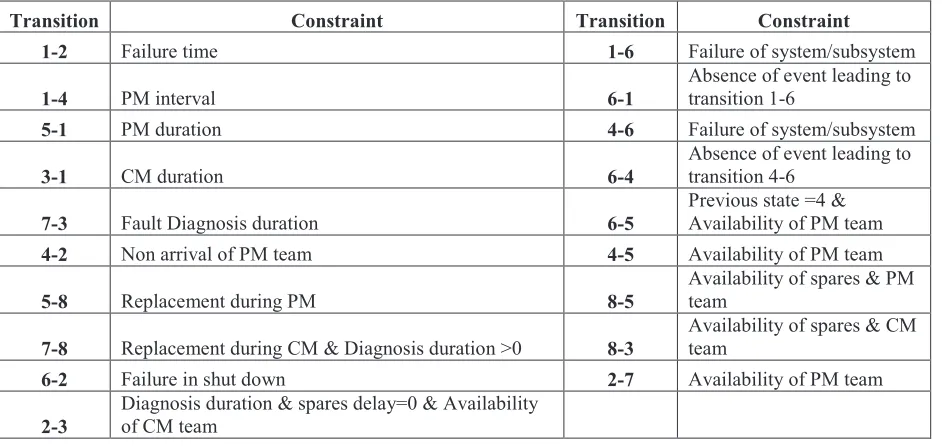
Division VIII Conditional transitions only occur when certain requirements are fulfilled. The underlying distributions of forced and conditional transitions are normally unknown prior to system analysis and are therefore not required. Table 2 outlines the properties of these transitions.
Transition Constraint Transition Constraint
1-2 Failure time 1-6 Failure of system/subsystem
1-4 PM interval 6-1
Absence of event leading to transition 1-6
5-1 PM duration 4-6 Failure of system/subsystem
3-1 CM duration 6-4
Absence of event leading to transition 4-6
7-3 Fault Diagnosis duration 6-5
Previous state =4 & Availability of PM team
4-2 Non arrival of PM team 4-5 Availability of PM team
5-8 Replacement during PM 8-5
Availability of spares & PM team
7-8 Replacement during CM & Diagnosis duration >0 8-3
Availability of spares & CM team
6-2 Failure in shut down 2-7 Availability of PM team
2-3
Diagnosis duration & spares delay=0 & Availability
of CM team
System Modelling
Normally a complex system may consist of subsystems which themselves may be made up of sub subsystems forming a hierarchical network. A similar hierarchical approach is followed in modelling the system. Subsystems are assigned IDs and ranks as a function of their hierarchical position in the network; level one being the subsystems closest to the system level as shown in Figure 2. Each subsystem is modelled as a multi-state object defined by the number of possible output levels the subsystem may exist
State Designation Definition
1 Working When the component operates at its required output level
2 Failed
Component is failed and corrective maintenance has not started, component output is zero.
3 CM Component is under repair; output is still zero
4 Awaiting PM
Component is due for preventive maintenance but PM hasn’t started; output is the same as in working
5 PM Preventive maintenance in progress; output is zero
6 Shut Down Component is not failed but it is not in operation; Output zero.
7 Diagnostic Failure is being diagnosed by maintenance team
8 Idle Diagnosis is complete and maintenance crew is waiting for spares
Table 1: State assignment for components
Figure 1. Component transitions
1
2
3
5 6
4
8 7
Table 2: Description of state transitions Forced Transitions
Division VIII in. Modelling of a subsystem is completed by defining cut-sets for each subsystem state and the output configuration based on its reliability block diagram. The system is defined using the subsystem and component objects according to its hierarchical network and effective block diagram.
The output configuration of the system or a subsystem is represented by a cell containing the IDs of its building block. Each position of the cell represents an element/block in series with parallel blocks represented by another cell containing two elements; an integer defining the minimum number of branches required for success and the second element an n by m matrix, where n is the number of branches in the block and m the number of elements in the longest branch. Each position in the matrix contains the ID of an element and the remaining positions in shorter branches filled with zeros. Equations 1 and 3 are expressions of the output ratio (ratio of current output to maximum output), X of a series, non-redundant parallel and r-out-of-k redundant block respectively.
ܺ௦௦ ൌ ሺܺଵǡ ܺଶǡ ǥ ǡ ܺሻ ܺ ൌ ݉݁ܽ݊ሺܺଵǡ ܺଶǡ ǥ ǡ ܺሻ
ܺௗ௨ௗ௧ൌ ͳ݂݅ݏݑ݉ሺܺଵǡ ܺଶǡ ǥ ǡ ܺሻ ݎܽ݊݀ܺௗ௨ௗ௧ൌ Ͳ݂݅ݏݑ݉ሺܺଵǡ ܺଶǡ ǥ ǡ ܺሻ ൏ ݎ
Where k is the number of components in the block, ܺ the output ratio of the ݇௧ component and r the minimum number of components required for success of the block.
Determining System/Subsystem States
The current state of the system or a subsystem is determined by evaluating the minimum and maximum cut sets defined for each state as proposed by Zio et al. (2006).
The minimum cut-set of an event, is the minimum combination of component unavailability/failure that lead to the occurrence of that event. The maximum cut-set on the other hand is the maximum combination of component unavailability/failure that could occur and still guarantee that the system/subsystem remains in its current state.
Since a system can only reside in one state at any instance, for an n state system/subsystem, cut sets are defined for ݊ െ ͳ states only, the ݊௧ state is determined from the logical expression in equation 4.
ܵൌ ܣܰܦሺܵଵᇱǡ ܵଶᇱǡ ǥ ǡ ܵିଵᇱ ሻ
In equation 4, ܵ is the logical value indicating the existence of the system in state n. Figure 2. Hierarchical structure of engineering systems
(2) (3) (1)
SUBSYSTEM 4 SYSTEM
SUBSYSTEM 3 SUBSYSTEM 2
SUBSYSTEM 1
C1 C2 C3 C4 C5 C6
Rank 1
Rank 1
Rank 2 Rank 2
Division VIII
Cost Analysis
The resultant effect of component failure, maintenance policy and external stochastic events on the system is expressed in terms of the average annual loss incurred. We propose equation 5 to compute this loss which as shown constitutes four partial losses.
· Loss due to lost output which in turn is due to system outages/partial outages consequent of component failure and maintenance.
· Fixed maintenance cost emanating from fixed wages for maintenance personnel.
· Cost of maintaining system components which is a function of time spent by each component in maintenance and the cost per hour of maintenance.
· Cost of spares used in maintaining system components.
ܣ݊݊ݑ݈ܽܮݏݏ ൌ ͺͲ ቂܹܥ൫ͳ െ ܿ൯ ݉ܰ ଵ
்ሺσ ݉ଵ ݐ σ ܿଵ ݏሻቃ
Where ܹ represents the maximum output of the system per hour,ܥ price per unit output of the system, ܿ the computed capacity factor of the system, ܶ the total period in hours for which the system is studied , ݉ fixed wage per maintenance persons per hour prorated over 24 hours, ܰ number of maintenance persons, ݉ cost of maintaining component n per hour, ݐ time spent by component n in maintenance, ܿ spares cost for component n, ݏ number of spares used for component n and ݊ the total number of components. The factor 8760 (there are 8760 hours in year) was introduced in equation 5 to adjust the total loss per hour to the annual level.
Key deliverables
In addition to the reliability indices of the system, the reliability indices of each component and subsystem are also determined. The computational tool;
· Can implement any transition probability distribution using the Open Cossan toolbox described by Patelli et al. (2014) to sample transitions between component states.
· Can analyse the system in any initial state, the system does not necessarily initially need to be in a working state.
· Can derive the distribution governing every transition at the component, subsystem and system levels.
· Provides the instantaneous/average output and availability of the system and components.
· Provides the time spent in each state
· Provides the number of spares used by each component.
· Provides maintenance cost per component
· Provides the transition map of the system/subsystems
Assumptions
The methodology and computational tool are subject to the following assumptions.
· When the system fails or is shut down, no components will fail until the system is restored.
· After preventive and corrective maintenance, the component/system is regarded as new.
· If preventive maintenance of a component is suspended as a result of unavailability of spares, then the component will remain out of operation and restored only after preventive maintenance.
Division VIII component to maintain is selected randomly according to a uniformly distributed random variable.
· The next state of a component depends on its current and previous states.
CASE STUDY: A TWO-UNIT 50MW HYDROELECTRIC POWER PLANT
Located at latitude 9o2’N and longitude 11o44’W northern Sierra Leone, the Bumbuna hydroelectric plant
is a two-unit 50MW plant that supplies power to the capital Freetown.
The methodology described was used to simulate the operation of a replica of the Bumbuna hydroelectric power plant for a period of 5 years. The reliability indices and performance of the plant for various maintenance policies were determined. The result of the analysis was used to select the most suitable policy based on high reliability, high energy output and low maintenance cost.
Figure 3 shows the schematic of the two unit hydroelectric power plant which reliability data is given in Table 3. It is important to note that a significant amount of the data was assumed given the difficulty in obtaining actual field data from the plant operator.
The plant analysis was subject to the following assumptions and underlying operating principles.
· The plant is new, therefore a component cannot fail whilst in shutdown
· Each unit of the plant is rated 25MW
· If one of the two transformers is unavailable, the turbine that has operated longer since the last preventive/corrective maintenance is shut down. This is a safety measure since the maximum rating of one transformer is less than the combined maximum output from the two turbines.
· The excitation unit and the generator are considered as one component; designated generator.
· The failure probabilities of the control gate and penstock are negligible thereby rendering them insignificant to the analysis.
Figure 3. Schematic of the Bumbuna Hydroelectric Power Plant
State Assignment
Division VIII Table 3: Component and system data
Note: All times are in hours and cost in kWh. Exp(m); an exponential distribution of mean ‘m’, W(x, y), U(x, y), Gu(x, y), G(x, y) & Log-N(x, y) respectively represent a Weibull, uniform, Gumbel, gamma and lognormal distribution with parameters x and y.
Table 4: State assignment for system
Network definition & reduction
Figure 4. Reliability block diagram of the Bumbuna Hydroelectric Power Plant
Figure 4 shows the reliability block diagram of the plant, where components 1 to 4 respectively represent Valve-1, Turbine-1, Generator-1 and Breaker-1, components 5 to 8 Valve-2, Turbine-2, Generator-2 and Breaker-2 and components 9 to 12 the synchronizing unit, Breaker-3, Transformer-1 and Transformer-2 respectively. To reduce the complexity of the plant, the reliability block diagram in Figure 4 was rearranged into subsystems as shown in Figure 5.
Subsystems A & B are made up of a series configuration of components (1, 2, 3 & 4) and (5, 6, 7 & 8) respectively. The minimum and maximum cut-sets of the system are as given in Table 5.
From Figure 4, one would expect the minimum cut sets for state 3 to be A, B, E and F contrary to the result given in Table 4. However, it could be recalled that when either E or F is unavailable, one of the
Component Valves Turbines Generators Breakers Synchronizer Transformers Failure Data W(4000,1.5) W(16500,2.1) W(8000,2) Exp(15000) Exp(13000) Exp(10000)
Repair Data Exp(20) Exp(53) Exp(75) Exp(18) Exp(48) Exp(40)
PM Interval U(2000,2500) U(4500,5000) U(4500,5000) U(8500,8700) U(8500,8700) U(8500,8700)
PM Duration Exp(4) Exp(10.6) Exp(15) Exp(3.6) Exp(9.6) Exp(8)
Diagnosis
Duration Exp(2.5) Exp(7) Gu(10,3.24) G(2.5,2) Exp(8) Log-N(8,2)
Spares Cost 812 1050 972 503 1122.5 1350
PM Cost/hr 52 78 65 32.5 78 84.5
CM Cost/hr 80 120 100 50 120 130
Spares Delay
CM 0.25 0.01 0.01 0.9 0.01 0.001
PM 0.1 0.003 0.003 0.42 0 0
Fraction 0.25 0.25 0.25 0.25 0.25 0.25
Log-N(3,1.21)
Probability of Component Replacement
Mean Fraction of PM Duration To Elapse Before Component Replacement becomes eminent
State Designation Definition
1 Working When the system operates at its required output level. 2 Failed System is failed, output is zero
Division VIII
400 410 420 430 440
3 4 5
Case
With Priority
Without Priority
State Minimum Cut Set Maximum Cut Set Subsystem State Minimum Cut Set Maximum Cut Set
1 None None A 2 1,2,3,4 1&2&3&4
2 C,D,EF,AB ABCDEF B 2 5,6,7,8 5&6&7&8
3 A,B AE,AF,BE,BF
System Subsystems
subsystems (A or B) will be shut down as a safety measure. This means the unavailability of E or F implies the unavailability of A or B, thereby satisfying the minimum cut sets A, B.
Figure 5. Reduced plant reliability block diagram
Analysis Procedure
The system was analysed for the following maintenance policies and the simulation results recorded.
· CASE 1: Non repairable
· CASE 2: Non repairable with preventive maintenance
· CASE 3: Repairable without preventive maintenance
· CASE 4: One team for both preventive and corrective maintenance. This was repeated for 2, 3 and 4 teams respectively giving rise to CASES 5 to 7.
· CASE 8: No restriction on the number of parallel maintenance actions
CASES 5 to 7 were repeated for dedicated maintenance in which case 50% of the team was dedicated to each maintenance type respectively giving rise to CASES 9 to 11. The scenario requiring three teams for dedicated maintenance was implemented as follows; two teams each dedicated to preventive or corrective maintenance and the remaining team handling both maintenance types. Each case (with the exception of Case1) was evaluated for both priority and non-priority maintenance.
RESULTS
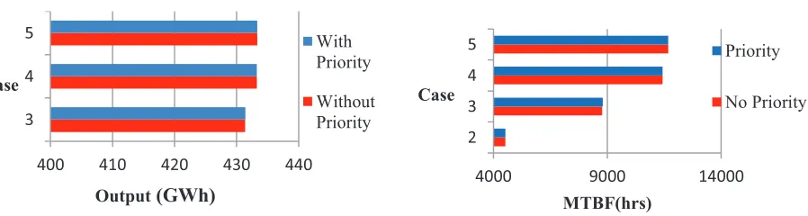
Outcomes of the analysis on the plant are presented in Table 6 and Figures 5 to 9.
4000 9000 14000
2 3 4 5
MTBF(hrs) Case
Priority
No Priority
Table 5: System/Subsystem Cut Sets
Figure 6. System Output for various cases A
B
C D
E
F
Division VIII
4 4.5 5
2 3 4
Loss(GWh) Number
of Teams
Loss(GWh) Dedicated
Loss(GWh) Shared
3 4 5 6 7 8 9 10 11
4.5 5 5.5 6 6.5 7
CASES
L
O
S
S
(G
W
h
)
CASE 1 2 3 4 5
ANNUAL LOSS(GWh)
No Priority
418.3842 412.1773 6.645072 4.779559 4.727691
Priority 412.1905 6.636802 4.780571 4.727747
Results for cases 6 to 11 are not shown because they are very close to the results for case 5.
Discussion of Results
It was observed that the Mean Time Between Failure (MTBF) and annual energy output improve with adoption of maintenance. There was a slight improvement in the MTBF with the adoption of preventive maintenance only and about 100% with corrective maintenance. This is so because a component after failure is repaired and restored as a new component, therefore the combination of component failures that lead to system failure will occur only after a relatively longer period. Hence the increase in MTBF and energy output of the system. However, moderate improvements in MTBF and energy output relative to case 3 were realised when both preventive and corrective maintenance (by a single team) were adopted. The levels remained unchanged when the number of maintenance teams was increased (see Figures 6 and 7). The plant’s energy output and MTBF remaining almost constant with increase in number of maintenance teams could be explained by the high reliability (low failure probability) of the plant’s
components. The same explanation accounts for the unexpected performance of the plant under priority maintenance. Priority maintenance proves useful in instances of high failure probability and/or inefficient maintenance team such that effective maintenance cannot be comfortably carried out by one team thereby imposing the need for preferential maintenance where critical components are placed high on the scale. The unexpected performance was exacerbated by the fact that only two (BREAKER-3 and SYNCHRONIZING UNIT) of the twelve components making up the system are critical (criticality of 1), the remainder have the same criticality value of 2. Hence priority maintenance wouldn’t have made much
difference even with a relatively inefficient maintenance team.
With reference to the simulation results and subsequent observations noted therein, the following conclusions could therefore be made.
· The reliability and performance of the plant depend on the type and quality of maintenance policy adopted but a threshold number of maintenance teams exists beyond which reliability and performance become independent of the number of teams implementing this policy assuming
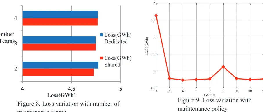
Figure 8. Loss variation with number of maintenance teams
Figure 9. Loss variation with maintenance policy
Division VIII fixed maintenance efficiency. The decision therefore to increase the number of maintenance teams depends on whether the gains from reduced spares/replacement cost out way the losses from reduced plant output and increased wages (maintenance personnel) .
· MTBF and plant output only do not tell the whole story, a third indicator (Loss) is required for a rational decision making process as shown in Figure 9.
· For multiple maintenance teams, dedicated maintenance is disadvantageous as shown is Figure 8. With reference to Figure 9 and Table 6, the best maintenance policy for the plant is shared preventive and corrective maintenance carried out by two teams (Case 5).
MERITS AND LIMITATIONS
In addition to the merits already discussed, this approach requires fewer samples and less time when compared to traditional Monte Carlo Simulation techniques. A huge chunk of memory is required for large systems as a consequence of keeping simulation history of components and subsystems. Due to the way the output configuration of systems/subsystems is defined, only series, parallel and series-parallel configurations can be implemented by this algorithm. However, research to surmount these limitations is underway.
CONCLUSIONS
We have successfully shown that the algorithm developed can be used to evaluate the response of a realistic multi component, multi output complex engineering system to a series of restrictive maintenance policies and is applicable to both continuous and mission oriented (non-repairable) systems. Components can be multistate with any failure/repair distribution and the results obtained can aid effective decision making in the maintenance planning process.
ACKNOWLEDGEMENTS
We appreciate the COSSAN working group of the University of Liverpool and the Centre for Doctoral Training on Quantification and Management of Risk and Uncertainty in Complex Systems and Environments for their resources and training.
REFERENCES
[1] Cristina, H., Simona, D. (2009). “Research on the Reliability Modelling of Hydro Mechanical Systems”. Journal of Engineering Annals of Faculty of Engineering Hunedoara. 3, p312-317
[2] Denson, W. (1998). “The History of Reliability Prediction”. IEEE TRANSACTIONS ON RELIABILITY. 47 (3), P321-328.
[3] Majeed, A.R. & Sadiq, N.M. 2006, "Availability and reliability evaluation of Dokan Hydro Power Station", 2006 IEEE PES Transmission and Distribution Conference and Exposition:
[4] Patelli, E., Broggi, M., de Angelis, M. & Beer, M. (2014). “OpenCossan: An efficient open tool for dealing with epistemic and aleatory uncertainties”.Vulnerability, Uncertainty, and Risk. ASCE. pp. 2564-2573.
[5] Reliability Analysis Center. (2003). Application of Markov Analysis Methods to Reliability, Maintainability and Safety. START. 10 (2), p1-8.
[6] Saleh, J.H., Marais, K. (2006). "Highlights from the early (and pre-) history of reliability engineering", Reliability Engineering & System Safety, vol. 91, no. 2, pp. 249-256.