Abstract
Nay, D. Todd. Predicting Trunk Kinematics from Static Task Parameters. (Under the direction of Dr. Gary A. Mirka.)
Many of the current ergonomic assessment tools available to industry take static “snapshots” of manual material handling (MMH) tasks to assess the hazards of a job. These tools are valuable to industry in that they provide a quick and inexpensive assessment of the task. However, these tools do not evaluate the trunk kinematics occurring during the task. As previous research has shown, trunk kinematics play an important role in assessing the stress placed on a person’s low back. The goal of this study was to provide a model that predicts the trunk kinematics as a result of static task
parameter inputs.
Biography
David Todd Nay was born May 24, 1971 in Rock Island, Illinois. His family moved to the Washington, D.C. area in 1975, where he graduated from high school in June 1989. After high school, Todd enrolled at Virginia Tech, graduating with a Bachelor of Science in Ocean Engineering in May 1994. After graduation from Virginia Tech, Todd worked as a reliability engineer in Washington, D.C.
Todd started his graduate studies in Industrial Engineering at North Carolina State University in the fall of 1997. His concentration has been Ergonomics, with a minor in Interdisciplinary Studies. His area of interests has been in the field of occupational
Contents
LIST OF TABLES V
LISTS OF FIGURES VI
LISTS OF EQUATIONS VII
1 INTRODUCTION 1
1.1 LOW BACK WMSDS 2
1.2 RISK FACTORS FOR LOW BACK WMSDS 2
1.3 METHODS OF ANALYZING JOBS FOR INJURY POTENTIAL 4
1.3.1 COMPUTER-AIDED SYSTEMS 4
1.3.2 MANUAL SYSTEMS 6
1.4 THE ROLE OF TRUNK DYNAMICS 12
1.5 TRUNK MOTION PREDICTION STUDIES 15
1.6 STUDY OBJECTIVE 18
2 METHODS 19
2.1 SUBJECTS 19
2.2 EXPERIMENTAL DESIGN 20
2.2.1 INDEPENDENT VARIABLES 20
2.2.2 DEPENDENT VARIABLES 21
2.2.3 EXPERIMENTAL DESIGN 21
2.3 EQUIPMENT 22
2.3.1 LUMBAR MOTION MONITOR 22
2.3.2 HEART RATE MONITOR 24
2.3.3 ASYMMETRIC REFERENCE FRAME 24
2.3.4 EXPERIMENTAL LIFTING ENVIRONMENT 25
2.4 EXPERIMENTAL PROCEDURES 28
2.5 DATA PROCESSING 31
2.5.1 LMM DATA PROCESSING 31
2.5.2 HEART RATE MONITOR 41
2.5.3 ASYMMETRIC REFERENCE FRAME 41
3 RESULTS 43
3.1 FINAL DATA MODEL 43
3.1.1 SAGITTAL PLANE MODELS 45
3.1.2 CORONAL PLANE MODELS 46
3.1.3 TRANSVERSE PLANE MODELS 47
3.2 VALIDATION OF THE MODEL 48
4 DISCUSSION 56
4.1 EQUATION DEVELOPMENT METHODOLOGY 56
4.2 MODEL VALIDATION 62
4.3 LIMITATIONS 66
4.4 FUTURE WORK 66
5 CONCLUSION 68
6 LITERATURE CITED 70
APPENDIX A: INFORMED CONSENT FORM 73
APPENDIX B: DATA VALIDATION ALGORITHM 77
List of Tables
TABLE 1. SUBJECT POPULATION INFORMATION 19
TABLE 2. LIST OF POSSIBLE REGRESSION PREDICTORS 40
Lists of Figures
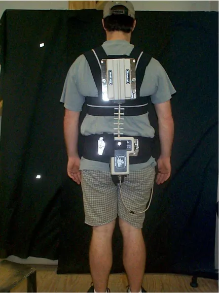
FIGURE 1. LMM BEING WORN BY A SUBJECT. 23
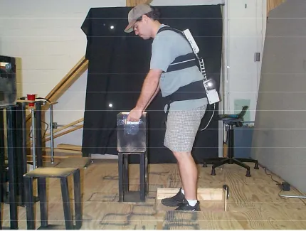
FIGURE 2. LIFTING STATION WITH BOX ON THE GROUND. 26
FIGURE 3. LIFTING STATION WITH BOX ON A STAND. 27
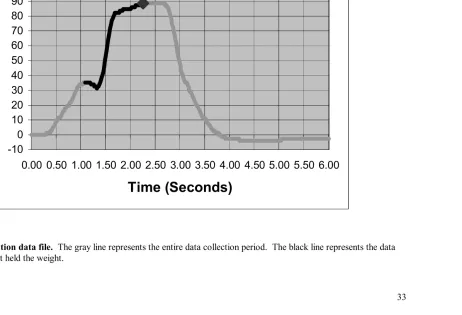
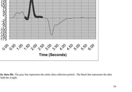
FIGURE 4. GRAPH OF POSITION DATA FILE. 33
FIGURE 5. GRAPH OF VELOCITY DATA FILE. 34
FIGURE 6. GRAPH OF ACCELERATION DATA FILE. 35
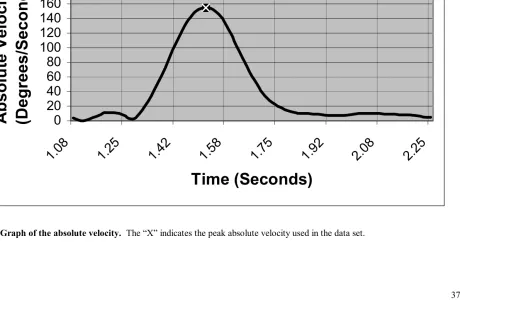
FIGURE 7. GRAPH OF THE ABSOLUTE VELOCITY. 37
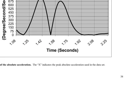
FIGURE 8. GRAPH OF THE ABSOLUTE ACCELERATION. 38
FIGURE 9. ACTUAL VS. PREDICTED PHRGM FOR EVERY LIFT 49
FIGURE 10. ACTUAL VS. PREDICTED PHRGM FOR LIFTS THAT DO NOT
GO THROUGH THE MID-SAGITTAL PLANE 50
FIGURE 11. ACTUAL VS. PREDICTED PHRGM FOR LIFTS THAT GO
THROUGH THE MID-SAGITTAL PLANE 51
FIGURE 12. ACTUAL VS. DIRECT PHRGM FOR EVERY LIFT. 53
FIGURE 13. ACTUAL VS. DIRECT PHRGM FOR LIFTS NOT THROUGH THE
MID-SAGITTAL PLANE. 54
FIGURE 14. ACTUAL VS. DIRECT FOR LIFTS THAT GO THROUGH THE
Lists of Equations
EQN. 1 SAGITTAL POSITION 45
EQN. 2 SAGITTAL VELOCITY 45
EQN. 3 SAGITTAL ACCELERATION 45
EQN. 4 CORONAL POSITION 46
EQN. 5 CORONAL VELOCITY 46
EQN. 6 CORONAL ACCELERATION 46
EQN. 7 TRANSVERSE POSITION 47
EQN. 8 TRANSVERSE VELOCITY 47
EQN. 9 TRANSVERSE ACCELERATION 47
EQN. 10 AVERAGE TRANSVERSE VELOCITY 48
1 Introduction
In November of 2000 the United States Occupational Health and Safety
Administration (OSHA) issued a final Ergonomics Program standard (OSHA, 29 CFR 1910.900). The purpose of the standard was to “address the significant risk of employee exposure to ergonomic risk factors in jobs in general industry workplaces” (OSHA 2000 p.68262). This standard was a result of OSHA’s extensive review of the scientific
evidence on work-related musculoskeletal disorders (WMSDs) and the economical cost of these injuries to American businesses.
As a result of their review, OSHA determined that “(1) There is a positive
relationship between work-related musculoskeletal disorders and employee exposure to workplace risk factors, and (2) ergonomics programs and specific ergonomic interventions can substantially reduce the number and severity of these injuries” (OSHA 2000 p.68263). In studying the economic effects of WMSDs, OSHA determined that they account for one-third of all occupational injuries and illnesses reported to the Bureau of Labor Statistics (BLS) and one out of three dollars spent for workers’ compensation. This results in an annual cost to American businesses in excess of $15 billion.
OSHA in its 10-year study has shown the tremendous impact of WMSDs on American workers and the advantages of ergonomics in reducing workplace injuries.
1.1 Low Back WMSDs
WMSDs can affect the neck, shoulders, elbows, wrists, fingers, back, knees, ankles, and feet. However, the most costly and most prevalent body part affected is the lower back. The incidence of low back WMSDs in the United States work force has become a major problem for industry and insurance companies. In a summary of epidemiological studies, Andersson (1984) found prevalence rates ranging from 12.0 % to 30.2 %. Additionally, ranges of lifetime incidence were 48.8 % to 69.9%. Webster and Snook (1994) reported that 16% of all workers’ compensation claims were a result of low back WMSDs. The low back pain claims accounted for 33% of all claim costs. The total costs for all low back WMSD claims was found to be divided into 32.4% for medical costs and 65.8% for indemnity costs. Due to these factors, industry has been working to identify methods of reducing low back WMSDs.
1.2 Risk Factors for Low Back WMSDs
“Convincing evidence from the confluence of many investigations on biomechanical models, laboratory research and epidemiology studies that work related risk factors including (1) heavy physical work, (2) lifting and forceful movements, (3) bending, twisting, and awkward positions, and (4) static work positions ... can increase the risk of back disorder[s]” (OSHA 2000 p. 68483).
In addition to the risk factors identified in OSHA’s proposed standard, Marras et al. (1993) illustrated the importance of the dynamics of the torso in relation to low back injury risk. Specifically, Marras et al found that five task parameters could be used to distinguish between manual material handling (MMH) tasks which were classified as having a low or high risk of causing low back disorders. These parameters include the lifting frequency, load moment, trunk lateral velocity, trunk twisting velocity, and the trunk sagittal position.
These risk factors are all common in general industry. They are especially
common in MMH work. If a work environment could be designed to reduce or eliminate an employee’s exposure to these risk factors, it would help to reduce their probability of incurring a low back WMSD. This has been shown in numerous ergonomic intervention studies reviewed by OSHA for their proposed standard. In their review of case studies on the effectiveness of ergonomic programs, OSHA found that “ergonomic programs
designed to reduce exposures to biomechanical risk factors do reduce the incidence of [W]MSDs in exposed workers” (OSHA 2000, p. 68570).
Ergonomists must understand the risk factors present during the work, the amount of time employees will spend performing the work, the types of tools used, and the
work being performed. Collecting and understanding this information will help ergonomists design work environments that eliminate or reduce low back WMSDs.
1.3 Methods of analyzing jobs for injury potential
1.3.1 Computer-Aided Systems
Ergonomists have used a variety of methods to evaluate workstation design over the years. One of the primary methods used has been workstation mock-ups in which human subjects would evaluate the layout by performing various tasks (Woodson, 1992). A second method is a simple scaled model. Cardboard manikins are placed in the model to help ergonomists determine the workstation layout from a reach perspective. Both of these methods are effective, but their use is limited due to the costs and time associated in building them. Due to the modeling time and cost factors, it is often not possible to make a change to the design and then make a new model for reevaluation.
changes can be made earlier in the design process and quickly reevaluated prior to the development of costly mock-ups.
The current problem with CAE, however, is how the movement of the human model is determined. Most of the programs require the user to input the changes in posture. This is completed through the operator picking a successive series of points in space that a specific body part will move through. The CAE software then uses a database of joint angles to determine the posture of the human model throughout the movement. This method can be time consuming because it requires so many inputs by the operator. It can also be inaccurate, since it is relying on the operator’s experience to properly identify the movement of the human model
One possible method to improve the accuracy of human model movement and to reduce the time necessary to perform sampling methods would be the use of posture prediction programs. Bernard (1993), Dysart and Woldstad (1996), Ayoub (1997), Woldstad (1997) from Texas Tech University have worked together to develop a program that predicts two-dimensional postures during lifting tasks. The program requires the user to input the position of the hands, the position of the feet, and anthropometric information about the subject in order to predict the position of the knee, hip, shoulder, and elbow joints in the sagittal plane. Their model first determines all of the possible postures, and then selects the optimal posture by minimizing overall effort, fatigue, and maximizing stability. This is all done through the calculation of the torque across the joints. The Texas Tech model, however, has only met with mild success at predicting postures
performed by the subjects. Subjects performed a squat, stoop, or a mixture of these methods in lifts from the ground. Researchers found that the predicted values were much more representative of a stooped lift.
One shortcoming of many posture prediction models that limits their usefulness in CAE is that they do not predict posture in all three planes of the body (sagittal, coronal, and transverse). In the real world, movement is three-dimensional. When modeling in CAD, it is done in a three dimensional environment. Utilizing the results from a two dimensional model would limit its usefulness in the CAE program. A two-dimensional model would additionally eliminate the evaluation of asymmetric postures, which were listed above as a risk factor for low back WMSDs. A more useful posture prediction model would provide posture and kinematics information in all three planes.
1.3.2 Manual Systems
In addition to evaluating workstation designs before they are built, ergonomist also evaluate jobs as they are currently being performed. This is to determine whether the design of the job could be a causative factor in worker injuries. When evaluating a current job, ergonomists evaluate the presence of the previously mentioned risk factors for low back WMSDs. These evaluations can be performed through the use of ergonomic assessment tools. Ergonomic assessment tools usually involve either work sampling or work evaluation methods.
This usually involves an observation on the posture that the legs, back, neck, arms, and wrists are in during the work-sampling interval. Usually an observation on the amount of weight the worker is handling and the duration of the work is recorded. Two of the most common work-sampling methods are OWAS (Karhu et al 1977) and RULA (McAtamney, 1993).
The Ovako Working Posture Analyzing System (OWAS) developed by Karhu et al. (1977) is a simple method of analyzing postures. The OWAS system requires an observer to make several instantaneous samples of the worker’s posture. The posture is described using four codes that indicate the position of the worker’s upper extremities (three levels), lower extremities (seven levels), the back (four levels), and the force. Using the four-position code, ergonomist can determine whether a job is hazardous or not and whether it should be redesigned. The major advantage of the OWAS method is that it is simple and only takes a few seconds to perform. The major disadvantage of the OWAS method, however, is the low resolution achieved in defining the postures worked.
Another disadvantage of the OWAS system is the inability to evaluate the dynamic nature of the postures involved with a job.
inserted into a series of exertion tables with the output resulting in a recommended course of action for the task. The recommended course of actions range from “no change to the job necessary” to “change the job immediately.” The primary advantages of the RULA method over the OWAS method are the higher resolution in the definition of the posture and the evaluation of static postures. The primary disadvantage of the RULA method is the significantly longer amount of time to complete an analysis while still not addressing the dynamics of the activity.
The second variety of ergonomic assessment tools involves work evaluation methods. Work evaluation methods involve gathering measurements of a work place and then using that information to perform a biomechanical analysis of the worker performing the job. The biomechancial analysis estimates whether the job requirements exceed safe lifting limits. Two of the most common methods of work evaluation are the University of Michigan’s 3-D Static Strength Prediction ProgramTM (3DSSPP) (Chaffin, 1991) and the National Institute for Occupational Safety and Health’s (NIOSH) Revised Lifting
Equation (Waters et al 1993).
3-modeling software. The following are the required inputs to the 3-dimensional biomechanical model:
• Joint angles of the upper arm, forearm, torso, the upper and lower leg,
• Height and weight of the worker,
• Weight of the object being lifted.
Using the biomechanical model, the 3DSSPP calculates the torque at the elbow, shoulder, torso, hip, knee, and ankle joints. It then compares the required torque values to an anthropometric static strength database. The outcome of the 3DSSPP is a percentage of the working population capable of generating those levels of torque. The primary advantage of the 3DSSPP is the fact that it analyzes lifts based upon strength
requirements. Studies have shown that there is a high increase in worker injury when workers are required to exceed their strength capabilities (Chaffin, 1974). Chaffin (1974) found a three-fold increase in low back WMSD incidence rates when workers exceeded their strength capabilities. The primary limitation of the 3DSSPP is the fact that it does not address the risks posed by highly repetitive tasks. These tasks, while not exceeding a worker’s strength capabilities in a single lift, can still result in low back WMSDs due to the repeated loading of the spine.
3DSSPP, the revised NIOSH lifting equation can assess the risk associated with repetitive MMH lifting tasks.
In creating the revised lifting equation, NIOSH used criteria developed from biomechanical, physiological, and psychophysical research to develop the concept of a standard lift. The standard lift is defined as a lifting location that is directly in front of a worker at a height of 75 cm above the floor and 25 cm from the mid-point between the worker’s ankles. The standard lift would be performed occasionally throughout the day and would involve moving a container having good coupling and a vertical travel distance less than or equal to 25 cm. It was determined that this standard lift could be performed with a load constant (LC) of 23 kg and still be acceptable to 90% of a mixed gender population. Deviations from the standard lift, however, would result in a recommended weight limit (RWL) for the lift being less than the LC in order for the lift to remain acceptable to 90% of the mixed gender population.
The revised NIOSH lifting equation calculates the acceptable weight
quality of the hand coupling (CM). The multipliers range in value from 0 to 1 and thus never result in the RWL being greater than the LC.
An RWL is calculated for the beginning and ending points of the lift with the lower value being used as the RWL for the MMH task. The ratio of the actual load to the RWL is called the Lifting Index (LI). A LI value less than 1 is ideal. LI values between 1 and 3 indicate an increased level of low back WMSD risk. LI values greater than 3 indicate a significant increase in low back WMSD risk (Waters 1993).
The revised NIOSH lifting equation is a valuable asset for ergonomists assessing the risk of low back WMSD associated with MMH lifting tasks. The equation has a simplified set of input variables that are easily collected with only a ruler, stopwatch, and a goniometer. It is also helpful for ergonomists that the output of the equation provides a specific weight limit for the lifting task being analyzed. In addition, the revised NIOSH lifting equation provides a method of assessing the relative level of hazard associated with a lifting task which allows tasks that need to be changed to be prioritized.
Essentially, all of the previously mentioned ergonomic assessment tools take a static “snapshot” of the manual material handling tasks to assess the hazards of a job. These tools are valuable to industry in that they provide a quick and inexpensive assessment of the task. While the assessment tools are fairly easy to use and they provide information as to the risk associated with a lifting task, the tools do not consider the trunk dynamics that occur during the task.
1.4 The Role of Trunk Dynamics
Research has shown that the trunk dynamics play an important role in assessing the stress placed on a person’s low back (Bigos et al, 1986; Freivalds et al, 1984; McGill and Norman, 1985, OSHA 2000). Therefore, it is important for ergonomic assessment tools to also consider the trunk dynamics of MMH tasks. Researchers at The Ohio State University developed a low back WMSD risk assessment model which was developed through a multiple logistic regression of historical injury data and trunk kinematics data collected from workers performing 403 industrial tasks (Marras et al. 1993). The tasks were classified as having either a low, medium, or high risk of low back WMSD based upon injuries and employee turnover rates. The results showed that the lift frequency, the maximum sagittal angle, the average twisting velocity, the maximum lateral velocity, and the maximum moment that occurs during a lifting task were the best predictors to
good predictor of low back WMSDs, however, it does require the knowledge of trunk kinematics associated with a task (OSHA, 2000).
The primary limiting factor of The Ohio State University model is the method required to collect the trunk kinematics data. To collect that data requires special
equipment and expertise not readily available to industry. In addition, workers must wear the equipment while they work which may result in postural changes from their normal methods (LI 1999). Additionally, the model was developed to evaluate the trunk dynamics involved with a MMH lifting task. Mirka et al (2000) verified that The Ohio State University model was limited in its ability to assess the risks in tasks that were static or that had high-forces associated with them. They suggest that this assessment tool should be used in conjunction with the 3DSSPP and the Revised NIOSH Lifting Equation to generate overall appreciation for the risks posed by an MMH task.
The continuous assessment of back stress (CABS) methodology developed by Mirka et al (2000) utilizes the revised NIOSH lifting equation, the 3DSSPP, and The Ohio State University Model to provide a comprehensive assessment of the low-back WMSD risk associated with MMH tasks. In their study, they found that each of the methods, while valuable in identifying certain types of MMH tasks as having a high-risk of low back WMSD, they are not able to fully identify every high-risk task. This result supported the research findings of Lavender et al. (1999) which also evaluated these same three
ergonomic assessment tools. Lavender et al used each of the three ergonomic assessment tools to analyze the low back WMSD risks associated with production jobs. Their
should be one of many ergonomic assessment tools used during an ergonomic analysis rather than the only tool used.
The CABS methodology consisted of three stages of analysis. The first stage
consisted of videotaping common tasks performed in the home construction industry. The second stage consisted of a continuous coding of the videotape data. The coding system was developed specifically for the CABS methodology analysis of the home construction industry and described the worker’s posture, action, and the weight they were handling on a continuous basis. The third stage consisted of laboratory simulations of the codes recorded in the second stage. The laboratory simulations allowed for the collection of data to input into the three ergonomic assessment tools.
The completed CABS analysis provides ergonomists with a more accurate
1.5 Trunk Motion Prediction Studies
Several researchers have developed regression models that attempt to predict trunk dynamics and which could be used as inputs to some of the models previously discussed. Ferguson et al (1992) developed models to predict the range of motion, peak velocity, average velocity, and peak acceleration in the sagittal, coronal, and transverse planes. The models are based upon data collected by Ferguson et al in a study which had subjects performing lifts from either a zero asymmetry position to a non-zero asymmetry position or from a non-zero asymmetry position to a zero asymmetry position. The independent variables in the study were the task asymmetry and the task weight. In the study, all of the non-zero asymmetry positions were to the right at 30), 60), 90), 120), 150) or 180). The study used three different weights: 14, 28, and 42 pounds. The horizontal distance (19 in.), vertical height (18 in.), vertical distance traveled (24 in.), and the lifting frequency (1 lift/min) were kept constant.
Ferguson et al reported significant R2 values at the 0.05 level for their models that
could predict the sagittal, coronal, and transverse range of motions and average velocities. The sagittal, coronal, and transverse range of motion R2 values were 0.83, 0.63, and 0.98,
respectively. The average velocities had R2 values of 0.87, 0.66, and 0.87, respectively.
The models to predict the sagittal and transverse peak velocities and peak accelerations gave large R2 values as well. The sagittal and transverse peak velocities had R2 values of
0.67 and 0.87, respectively. The sagittal and transverse peak accelerations had R2 values
of 0.81 and 0.98, respectively. The possible model variables were the linear and
Since the models require only the task asymmetry and weight as their inputs, the Ferguson et al models provide ergonomists with a simple method to obtain the necessary trunk dynamics for input into some of the previously discussed ergonomic assessment tools. The primary limitations in using the Ferguson et al models, however, are the range of motions for which the models were developed. During the experiment the vertical and horizontal distances did not change, similar to what would be seen if someone was moving items from one conveyor belt to another. For that type of tasks, the models would
perform well. However, the models would not be valid in tasks where the vertical and horizontal distances changed. One example of this from industry is the loading or unloading of pallets.
In another study, Harrison (1994) developed gender specific models to predict sagittal position, velocity, and acceleration given the starting height, the starting task asymmetry, and the task weight. Harrison’s models were developed for lifts that were started at heights from 25 to 65 cm and ended at the subject’s knuckle height. The lifts were started at either zero or 90 degrees asymmetry and finished at zero degree
asymmetry. The possible model variables were the vertical height, the asymmetrical distance and the weight.
The Harrison models reported R2 values that were lower than the Ferguson et al
would eliminate the ability of ergonomists to analyze asymmetric trunk kinematics. The small levels of task asymmetry and horizontal distances used in the experiment also limit the usefulness of the models to ergonomists who are looking at real world MMH tasks. Both the Ferguson et al and Harrison models are limited in their application to real world tasks due to their inability to evaluate lifting tasks that move through the zero asymmetry plane. An example of this would be the position a worker chooses when moving boxes from a conveyor to another surface. The worker could choose to face the first conveyor to lift the box and then turn their trunk 90 degrees to place the box down on another work surface. Or, the worker could choose to stand in between the two conveyors and turn their trunk 45 degrees to one side to pick up the box. The worker would then rotate their trunk through the zero asymmetry plane and place the box down on the surface at a 45 degree position on the other side.
1.6 Study Objective
While dynamic information about a lift can be helpful to field ergonomists evaluating lifting tasks, collecting that data can be time-consuming and costly. In comparison, the static measurements necessary for assessment tools like the Revised NIOSH Lifting Equation can be completed quickly and at minimal costs but may overlook important information with regard to risk. A model that combines the additional predictive strength provided by the analysis of the dynamic motions with the ease of collecting static
parameters would provide a more complete assessment tool for ergonomists.
2 Methods
2.1 Subjects
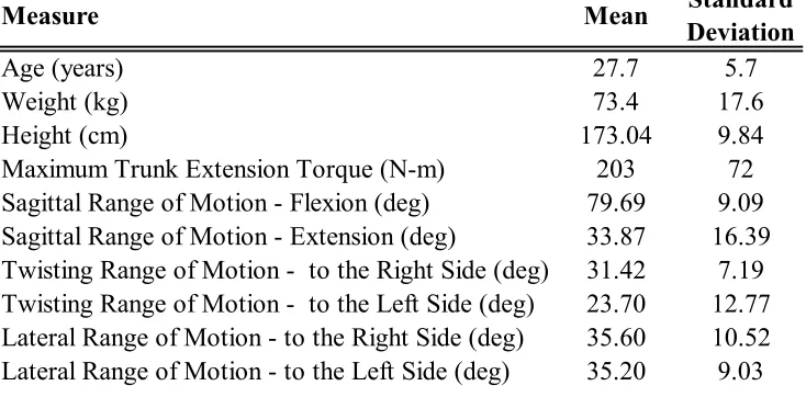
Thirty subjects participated on a voluntary basis for this study. The subject population consisted of 15 females and 15 males with no history of low back or knee injuries. Population information is summarized in Table 1.
Table 1. Subject population information
Measure Mean Standard
Deviation
Age (years) 27.7 5.7
Weight (kg) 73.4 17.6
Height (cm) 173.04 9.84
Maximum Trunk Extension Torque (N-m) 203 72
Sagittal Range of Motion - Flexion (deg) 79.69 9.09 Sagittal Range of Motion - Extension (deg) 33.87 16.39 Twisting Range of Motion - to the Right Side (deg) 31.42 7.19 Twisting Range of Motion - to the Left Side (deg) 23.70 12.77 Lateral Range of Motion - to the Right Side (deg) 35.60 10.52 Lateral Range of Motion - to the Left Side (deg) 35.20 9.03
Subjects were instructed as to the hazards involved with this study through an Informed Consent process approved by the Institutional Review Board for Human
Subjects of North Carolina State University. The subjects were free to withdraw from the study at anytime. Subjects received a North Carolina State University Ergonomics
2.2 Experimental Design
2.2.1 Independent Variables
The independent variables were set as the input variables of the NIOSH Lifting Equation (Waters, 1993):
1. Starting Asymmetry location of the box (5 levels) 2. Ending Asymmetry location of the box (5 levels) 3. Starting Vertical Height of the box (3 levels) 4. Ending Vertical Height of the box (3 levels) 5. Starting Horizontal Location of the box (2 levels) 6. Ending Horizontal Location of the box (2 levels) 7. Weight of the box (2 levels).
2.2.2 Dependent Variables
The dependent variables for this experiment were variables describing trunk kinematics during the lifting activity. These measurements were the maximum position, the absolute peak velocity, and the absolute peak acceleration of the lumbar trunk in the sagittal, coronal, and transverse planes.
2.2.3 Experimental Design
The experiment was a split plot design utilizing a central composite arrangement to reduce the number of lifts required by each subject without reducing the model’s
predictive power. The split plot variables assigned to a subject were the horizontal and vertical ending positions. This means that for every lift the subject performed, the subject lifted a box from a random starting position to the same horizontal and vertical ending positions. While the horizontal and vertical ending positions remained constant for every lift a subject performed, the ending asymmetry location was randomized.
2.3 Equipment
2.3.1 Lumbar Motion Monitor
The Lumbar Motion Monitor (LMM) (Chattecx Corp., Chattanooga, TN) was used to collect the trunk kinematics data during the lifting activities. The LMM is an
exoskeleton that is worn on a person’s back and is secured to the torso using a shoulder harness and a waist belt as shown in Figure 1. The harness and belt design allowed the subjects to wear the LMM without any impediment to their trunk motions. The
2.3.2 Heart Rate Monitor
A Polar Heart Rate Monitor System (Polar Electro Inc., Kempele, Finland) was used to record the subjects’ heart rate during the experiment. The system consisted of a sensor/transmitter that strapped around the subject’s chest. A watch worn by the
researcher received the transmitted information. The subject’s heart rate was read off of the watch and then recorded on paper.
2.3.3 Asymmetric Reference Frame
An Asymmetric Reference Frame (ARF) connected to a KIN/COM dynamometer was used to record the subject’s maximum trunk extension torque while in a static, sagittally symmetric, 30 degree flexed position (Marras et al 1989). The ARF’s design allows researchers to restrain the subjects’ lower extremity, thus only allowing for trunk motion. By centering the rotating arm of the KIN/COM at the subject’s L5/S1, it allowed for the collection of the trunk extension torque around the L5/S1. During data collection, the trunk extension torque value was read directly off of the KIN/COM screen by the researchers.
2.3.4 Experimental Lifting Environment
In order to keep the lifting environment consistent across subjects, a lifting station was built. The lifting station can be seen in Figure 2. Every subject performed his or her lifts in this lifting station. The station consisted of a platform where the boxes being lifted were placed and a recessed cutout area where the subjects stood.
2.4 Experimental Procedures
Subjects were required to attend a single session lasting approximately two hours. Prior to being asked to be a subject in the experiment, subjects were screened for previous back and knee injuries. Upon arrival for the experiment, subjects were given an overview of the experiment. This consisted of an explanation of the purpose of the experiment as well as fully explaining the operation and use of each piece of equipment used in the experiment. Subjects were then asked to sign the informed consent form, a copy of which can be found in Appendix A.
After subjects signed the informed consent form, anthropometric measurements were taken. Subjects were then outfitted with the heart rate monitor and their seated resting heart rate was taken. To ensure that subjects were properly warmed up, they were required to do an aerobic warm up and stretching. The aerobic warm up consisted of a brief jog through the research facility. The stretching exercises targeted the legs, the arms, and the lower back.
result. This continued for a total of three exertions, with a minute break between each attempt.
The LMM was then placed on the subject’s torso and fitted such that it did not limit their range of motion. After properly fitting the LMM on the subject’s back, the LMM was calibrated to the subject’s posture. The calibrations consisted of determining the LMM readings in the subject’s upright, or zero degree position, and their flexed, or ninety-degree position. The zero degree position was determined by measuring the subject standing in an upright, neutral position. The ninety-degree position was measured by having the subject bend at the waist to a position where the line connecting the
proximal head of the humerous and the greater trochanter were parallel with the floor. These calibration measurements were also taken after the forty-fifth and ninety-sixth lifts. This was done to quantify any gradual shifting of the LMM on the subject during the experiment.
Next, subjects were asked to perform 6 practice lifts. This was to ensure that they were performing the lift as requested and did not have any questions. Upon completion of the practice lifts, the subject’s heart rate was recorded again.
Upon completion of these preliminary tasks, the experiment’s data collection phase was started. The data collection phase consisted of having the subjects perform the 96 lifts while LMM data was collected. Other than the split plot variables (ending horizontal and asymmetry position), the task parameters for each lift were randomized for each subject. At the beginning of every lift, the subject could see the box location at the start of the lift and was told where the box was to be placed. The researcher then started
recording LMM data and prompted the subject to begin the lift. If the lift was not acceptable, the box was placed back in the starting position and the lift was performed again. The lift was not acceptable if the subject lifted a box to the wrong location or started the lift prior to the start of the LMM data collection. After confirming that the lift was done properly, the researcher would then setup the beginning and ending locations for the next lift. This procedure was repeated for the first 45 lifts. The lifts during the entire experiment were kept constant at 2 lifts per minute. After the 45th lift, the subject’s heart
Following the stretches, the subject’s resting heart rate was monitored. The time for their resting heart rate to return to the pre-experiment resting heart rate was recorded.
2.5 Data Processing
2.5.1 LMM Data Processing
The LMM collected data for a period of six seconds for each lift in the study. The collection period started the moment the researcher initiated the LMM recording process and then continued for six seconds. However, the actual time that the subject was holding the weight was less than the six seconds of data collected. In order to get more precise information, the data that was collected outside of the actual lifting of the weight was not included in the final data set. The reduction of the data files from the full six seconds to just the time when the weight was being lifted was completed through a series of
-10
0
10
20
30
40
50
60
70
80
90
100
0.00 0.50 1.00 1.50 2.00 2.50 3.00 3.50 4.00 4.50 5.00 5.50 6.00
Time (Seconds)
P
o
sition (Degr
ees)
-175
-150
-125
-100
-75
-50
-25
0
25
50
75
100
125
150
175
0.
00
0.
50
1.
00
1.
50
2.
00
2.
50
3.
00
3.
50
4.
00
4.
50
5.
00
5.
50
6.
00
Time (Seconds)
V
e
lo
ci
ty
(
D
eg
rees/
S
ec
-900
-750
-600
-450
-300
-150
0
150
300
450
600
750
900
0.00 0.50 1.00 1.50 2.00 2.50 3.00 3.50 4.00 4.50 5.00 5.50 6.00
Time (Seconds)
Accel
erati
on
(D
egrees/
Second/
Second)
0
20
40
60
80
100
120
140
160
180
1.08
1.25
1.42
1.58
1.75
1.92
2.08
2.25
Time (Seconds)
Abs
o
lut
e Ve
loc
it
y
(Degrees/Second)
0
75
150
225
300
375
450
525
600
675
750
825
1.0
8
1.2
5
1.4
2
1.5
8
1.7
5
1.9
2
2.0
8
2.2
5
Using a program written at the NC State Ergonomics Laboratory, the maximum and minimum values for each of the LMM variables were extracted from the resulting file. This program produced a report file listing each of the maximum and minimum values. The position data were then normalized relative to the 0 and 90 degree postures. This was achieved through the use of the previously mentioned normalization files.
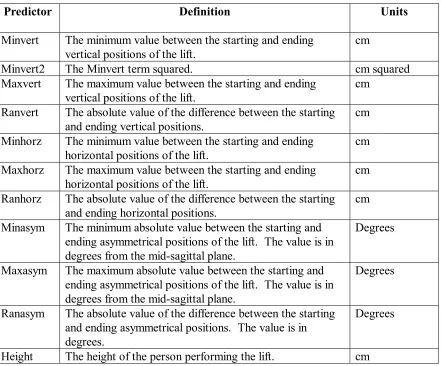
Table 2. List of possible regression predictors
Predictor Definition
Minvert The minimum value between the starting and ending vertical positions of the lift. Example: starting height is 35 cm, ending height is 76 cm. Use 35 cm.
Minvert2 The Minvert term squared.
Maxvert The maximum value between the starting and ending vertical positions of the lift. Example: starting height is 35 cm, ending height is 76 cm. Use 76 cm.
Ranvert The absolute value of the difference between the starting and ending vertical positions. Example: starting height is 35 cm, ending height is 76cm. Use 41 cm.
Minhorz The minimum value between the starting and ending horizontal positions of the lift. Example: starting horizontal position is 38 cm, ending position is 63 cm. Use 38 cm.
Maxhorz The maximum value between the starting and ending horizontal positions of the lift. Example: starting horizontal position is 38 cm, ending position is 63 cm. Use 63 cm.
Ranhorz The absolute value of the difference between the starting and ending horizontal positions. Example: starting horizontal position is 38 cm, ending position is 63 cm. Use 25 cm. Minasym The minimum absolute value between the starting and ending
asymmetrical positions of the lift. The value is in degrees from the mid-sagittal plane. Example: The starting asymmetrical position is –45 degrees, ending position is 90 degrees. Use 45 degrees.
Maxasym The maximum absolute value between the starting and ending asymmetrical positions of the lift. The value is in degrees from the mid-sagittal plane. Example: The starting asymmetrical position is –45 degrees, ending position is 90 degrees. Use 90 degrees.
Ranasym The absolute value of the difference between the starting and ending asymmetrical positions. The value is in degrees. Example: The starting asymmetrical position is –45 degrees, ending position is 90 degrees. Use 135 degrees.
Boxwght The weight being lifted during the task.
Weight Subjects weight.
Height The height of the person performing the lift.
Heart The time necessary for the subject’s heart rate to return to their pre-experiment’s resting heart rate.
MaxTorq The subject’s maximum extension torque measured by the ARF.
2.5.2 Heart Rate Monitor
The subject’s resting seated heart rate was recorded at the beginning of the experiment. The subject’s heart rate was then recorded after the 45th lift and after the last
lift. At the conclusion of the experiment, the subject’s heart rate was monitored to
determine the time it took to return to the pre-experiment’s resting seated heart rate. This information was used as a possible covariate in the regression equations to be described below.
2.5.3 Asymmetric Reference Frame
The information from the ARF was read directly off of the system’s monitor. The maximum value was then used as the subject’s maximum sagittal moment. This
information was also used as a possible covariate in the regression equations to be described below.
2.6 Model Validation
3 RESULTS
3.1 Final Data Model
This section presents the final regression equations, which form the model to predict the lifting trunk kinematics. There are regression equations to predict the peaks of
Table 3. Significant predictor variables
Predictor Definition Units
Minvert The minimum value between the starting and ending vertical positions of the lift.
cm
Minvert2 The Minvert term squared. cm squared
Maxvert The maximum value between the starting and ending vertical positions of the lift.
cm Ranvert The absolute value of the difference between the starting
and ending vertical positions.
cm Minhorz The minimum value between the starting and ending
horizontal positions of the lift.
cm Maxhorz The maximum value between the starting and ending
horizontal positions of the lift.
cm Ranhorz The absolute value of the difference between the starting
and ending horizontal positions.
cm Minasym The minimum absolute value between the starting and
ending asymmetrical positions of the lift. The value is in degrees from the mid-sagittal plane.
Degrees
Maxasym The maximum absolute value between the starting and ending asymmetrical positions of the lift. The value is in degrees from the mid-sagittal plane.
Degrees
Ranasym The absolute value of the difference between the starting and ending asymmetrical positions. The value is in degrees.
Degrees
3.1.1 Sagittal Plane Models
Equation 1 is the regression equation for the maximum sagittal flexion of the trunk. The equation had an absolute average error of 10.70 degrees and an R2 of 0.8137.
The complete statistical analysis for this equation and equations 2-11 can be found in Appendix C.
(Eqn 1) 24.95813 + 0.56752*HEIGHT + 0.20882*MAXHORZ – 1.69566*MINVERT + 0.00565*MINVERT2
Equation 2 is the regression equation for the maximum absolute sagittal velocity of the trunk. The equation had an absolute average error of 25.84 degrees per second and an R2 of 0.4955.
(Eqn. 2) –20.82954 + 0.43350*HEIGHT – 0.45962*MINVERT + 0.82451*RANVERT + 0.10104*RANASYM
Equation 3 is the regression equation for the maximum absolute sagittal
acceleration of the trunk. The equation had an absolute average error of 105.02 degrees per second squared and an R2 of 0.4291.
3.1.2 Coronal Plane Models
Equation 4 is the regression equation for the maximum absolute side-bending position of the trunk. The equation had an absolute average error of 3.23 degrees and an R2 of 0.1129.
(Eqn. 4) -19.06432 + 0.12711*HEIGHT – 0.01188*MINVERT + 0.03150*MAXASYM
Equation 5 is the regression equation for the maximum absolute side velocity of the trunk. The equation had an absolute average error of 5.50 degrees per second and an R2 of 0.0746.
(Eqn. 5) 12.26420 + 0.04403*MAXASYM – 0.06220*MINVERT + 0.02175*RANASYM
Equation 6 is the regression equation for the maximum absolute side acceleration of the trunk. The equation had an absolute average error of 22.09 degrees per second squared and an R2 of 0.0492.
3.1.3 Transverse Plane Models
Equation 7 is the regression equation for the maximum absolute rotational position of the trunk. The equation had an absolute average error of 4.21 degrees and an R2 of
0.0327.
(Eqn. 7) 1.17061 + 0.04437*MAXASYM + 0.01832*MINVERT
Equation 8 is the regression equation for the maximum absolute rotational velocity of the trunk. The equation had an absolute average error of 10.51 degrees per second and an R2 of 0.0551.
(Eqn. 8) -2.87346 + 0.06664*MINVERT + 0.10745*RANVERT + 0.09255*RANASYM
Equation 9 is the regression equation for the maximum absolute rotational acceleration of the trunk. The equation had an absolute average error of 43.05 degrees per second squared and an R2 of 0.0372.
3.2 Validation of the Model
In order to validate the current research’s model to predict trunk kinematics, the current research’s equations were used to provide input into the LMM Model. As previously discussed, the CABS data set developed by Mirka et al (2000) is used in this validation, however, only those lifts that were similar in scope to the ones performed during this study were used. Utilizing the CABS data set, all of the inputs into the LMM risk assessment model are either known or can now be predicted from the current
research’s model except for the average rotational velocity. That equation was also developed as part of this study and is presented in Equation 10. The equation had an absolute average error of 2.07 degrees per second and an R2 of 0.0620.
(Eqn. 10) -0.85821 + 0.01693*MINVERT + 0.03154*RANASYM + 0.04069*RANVERT
0
20
40
60
80
1
9
17
25
33
41
49
57
CABS Lift
Pr
o
b
a
b
ility o
f Hig
h
Risk
G
roup Me
mbe
rs
h
ip
Actual
Predicted
Figure 9. Actual vs. Predicted PHRGM for Every Lift
0
20
40
60
80
1
5
9
13
17
21
25
CABS Lift
Pr
o
b
a
b
ility o
f Hig
h
Risk
G
roup Me
mbe
rs
h
ip
Actual
Predicted
Figure 10. Actual vs. Predicted PHRGM for lifts that do not go through the Mid-Sagittal Plane
0
20
40
60
80
1
5
9
13
17
21
25
29
CABS Lift
Pr
o
b
a
b
ility o
f Hig
h
Risk
G
roup Me
mbe
rs
h
ip
Actual
Predicted
Figure 11. Actual vs. Predicted PHRGM for lifts that go through the Mid-Sagittal Plane
Another possible use of the data collected in this study would be the development of an equation to directly predict the LMM PHRGM (herein called “direct”). Equation 11 provides that prediction. The equation had an absolute average error of 4.19 and an R2
value of 0.3461.
(Eqn. 11) –3.78295 – 0.04210*MINVERT + 0.04957*RANASYM +
0.02693*RANVERT + 0.04678*MAXHORIZ + 0.31765*HEIGHT
0
20
40
60
80
1
8
15
22
29
36
43
50
57
CABS Lift
Pr
o
b
a
b
ility o
f Hig
h
Risk
G
roup Me
mbe
rs
h
ip
Actual
Direct
Figure 12. Actual vs. Direct PHRGM for Every Lift.
0
20
40
60
80
1
5
9
13
17
21
25
CABS Lift
Pr
o
b
a
b
ility o
f Hig
h
Risk
G
roup Me
mbe
rs
h
ip
Actual
Direct
Figure 13. Actual vs. Direct PHRGM for lifts not through the Mid-Sagittal Plane.
0
20
40
60
80
1
5
9
13
17
21
25
29
CABS Lift
Pr
o
b
a
b
ility o
f Hig
h
Risk
G
roup Me
mbe
rs
h
ip
Actual
Direct
Figure 14. Actual vs. Direct for lifts that go through the Mid-Sagittal Plane.
4 Discussion
The goal of this study was to develop a model that predicts trunk kinematics using the values of the inputs to the revised NIOSH lift equation. Those inputs consist of the
following: the beginning and ending vertical height, the beginning and ending horizontal distance, the beginning and ending asymmetrical location, and the weight of the object being lifted. Equations 1-9 represent the final models that predict the trunk kinematics given the above static task parameter inputs. The equations predict the maximum position, velocity, and acceleration in the sagittal, coronal, and transverse planes based upon these static task parameter input values.
4.1 Equation Development Methodology
The regression equations were developed through a process that considered both the statistical and biomechanical perspectives on the data. The biomechanical perspective was used to determine the factors that logically would impact a person’s lifting technique and the resulting kinematics parameters. Specifically, an understanding of the impact of the various task parameters on a person’s lifting posture and motion were incorporated into the equation development. The completed biomechanical prediction equation
statistically significant. In most cases, this resulted only in the elimination of the higher order terms from the biomechanical prediction equations.
During the development of the regression equations through the biomechanical methodology, it was important to understand the factors that would influence a person’s lifting posture. When determining the person’s posture during a lift, the location of the object to be lifted at the origin and destination plays a significant role. For example, the farthest distance away from the body in a plane has a significant effect upon the amount of flexion that occurs in that plane. Using this knowledge, the minimum values (the farthest distance from an upright position) of either the starting or ending vertical height were included. Similarly, the maximum value of the starting or ending horizontal distance and the maximum absolute value of the starting or ending asymmetrical position were
included. Review of the sagittal plane equations (Eqns. 1-3) in fact reveals that these variables were good predictors of sagittal plane kinematics.
the position, velocity, and acceleration in the coronal and transverse planes, however there was a significant effect in the sagittal plane.
When reviewing the data, there was a pattern of greater maximum flexion in the taller subjects than in the shorter subjects. Due to its influence on lifting posture, subject height was included in several of the equations. Analysis revealed that the height variable was statistically significant in some of the equations, particularly in the sagittal plane. Inclusion of the height variable was reasonable from a biomechanical sense as well, since the vertical task height was independent of subject height. As a result, taller subjects were farther away from the lower vertical task height, requiring them to travel through a greater range of motion than the shorter subjects.
The equations to predict the posture that were developed during the biomechanical methodology were used as the starting point in the equations to predict the trunk
kinematics. Added to the list of potential predictors for the position equations were variables that could have an effect on the trunk speed and acceleration during a lift. When determining the parameters which most influence the speed and accelerations that a person would lift with, it was determined that the distance the object was moved might play an important role. Therefore, in the biomechanical development of the equations to predict the velocity and acceleration in each plane, the range of vertical, horizontal, and
asymmetrical motion was included. It was believed that the greater the range of
The equation to predict posture in the sagittal plane (Eqn. 1) performed quite well and has a high R2 value indicating a good ability for predicting the posture. Ferguson et al
(1992) reported an equation to predict sagittal posture with a similar R2 value. Harrison
(1994) also developed models to predict male and female sagittal positions. The current model’s R2 was higher than both of those reported by Harrison. It should be noted that
the current study’s model has equal or greater predictive capability than the Ferguson et al and Harrison models over a much greater range of 3-D lifting configurations.
The current study’s equations to predict the peak sagittal velocity (Eqn. 2) and acceleration (Eqn. 3) did not have the same level of R2 values as the equation to predict
sagittal position. However, they did perform better than the current study’s equations to predict velocity and acceleration in the coronal and transverse planes. When comparing Equations 3 and 4 to other work the results were mixed. The Ferguson et al models achieved R2 values that were much higher than the current study’s R2 values. However, the Harrison models reported R2 values that were slightly lower. One possible reason for
this difference could be the number of different vertical heights used in each of the studies. The Ferguson et al study, which resulted in the highest R2 values, had subjects lift from a
single vertical height. The current study, which had the second highest R2 values of the three studies, had subjects lifting from three different starting heights. In comparison, Harrison’s study had five different vertical starting heights. The increased level of vertical starting heights would result in greater lifting motion variability. This increase in lifting variability would make it harder to accurately predict the trunk kinematics information. The R2 values for the equations to predict motion in the coronal and transverse
transverse and coronal planes can be quite difficult due to the high subject variability in the lifting motion. When a person has to lift an item, the sagittal motions they use in picking up the item are highly influenced by the vertical and horizontal location of the item as well as the height of the person. However, the motions in the transverse and coronal planes are much more dependent upon individual variability in technique. This is especially true when the object is not directly in front of them. If an object was to the side, the person could twist their trunk to pick up the item. Or, they could keep their trunk relatively straight and only bend over sideways to pick up the item. However, they could also use a combination of side bending and twisting. A person could also use various levels of pelvic twists when lifting weights that are not in front of them. It is this variability in the lifting methods that make it so difficult to accurately predict the rotational and transverse motions people will use when lifting.
Granata et al (1999) examined the variability of trunk kinematics, kinetics, and spinal loading during MMH tasks. Their study had subjects performing 10 repetitions of a MMH lifting tasks which involved two levels of box weight (13.6 and 27.3 kg), two levels of task asymmetry (0 and 60 degrees), and two levels of lifting velocity (preferred, and faster than preferred). They found that the variability in trunk kinematics was significantly dependent upon the task parameters, especially the task asymmetry. Granata et al
As a result, this would increase the difficulty of the current research’s model to accurately predict the trunk kinematics.
In general, the Ferguson et al (1992) model reported much higher R2 values for their
models in the three planes than those found in this study. However, as previously mentioned, their models are only valid for a small number of lifting combinations. They limited their study to a single level of task vertical height and horizontal position. In addition, all of their lifts started at the mid-sagittal plane and went to some angle of asymmetry. In contrast, this study used three levels of vertical height, two levels of horizontal distance, and allowed lifts to be performed from any of the task asymmetrical positions. So, while Ferguson et al would see some level of variation within a subject’s lifts, it would not be as high as what was seen in this study. Additionally, Ferguson et al reduced a significant amount of their subject’s variation by utilizing averaged values in the development of their models. Each of their subjects performed a specific lift three times. The results of these three lifts were averaged and used during their statistical analysis. This methodology would reduce errors due to the variability in lifting motions, as previously described by Granata et al.
4.2 Model Validation
While the model does not perform that well in the actual prediction of the coronal and transverse plane trunk kinematics during a lift, it is believed that the information can still be useful as input into other models which rely on trunk kinematics information in determining the risk of WMSDs. One such model, which has been previously discussed, is the LMM model. The LMM model uses the following five input variables: peak sagittal position, peak lateral velocity, average rotational velocity, frequency of lift, and maximum moment. The output of the model is the probability of high-risk group membership for a low back WMSD.
NIOSH Lifting Equation calculations and develop the LMM PHRGM. For this study, the CABS’ Revised NIOSH Lifting Equation inputs were used to predict the trunk kinematics information, which were then used as inputs to the LMM Model. The predicted PHRGM values were then compared to the CABS’ measured PHRGM values. A total of 57 lifts are used from the CABS data set. The 57 lifts were selected because they were similar to the lifts performed in this study.
In order to use the LMM model, a prediction for the average rotational velocity during a lift was also needed. In order to accomplish this, an additional regression equation was developed to perform this analysis. Equation 10 was developed to predict the average rotational velocity. In developing Equation 10, the same biomechanical methodology previously discussed was used. As a result, the average rotational velocity equation incorporated the same variables as the equation that predicted the maximum absolute rotational velocity (Equation 8).
The results of the comparison between the actual PHRGM to the predicted PHRGM can be seen in Figure 9. The average absolute error between the actual and predicted PHRGM is 8.07 percent. One interesting observation of the difference between the two probability values was the fact that the predicted values only went above 60 percent risk three times and in fact mainly predicted a probability of high risk group membership in the 50 percent range. This is a function of the types of lifts being evaluated.
After analysis of the results, the most significant trend observed was the
include the mid-sagittal plane. Figure 10 shows the actual PHRGM versus the predicted PHRGM for lifts that go through the mid-sagittal plane. As can be seen, the predicted values do a much better job on this data subset. The average absolute error between the actual PHRGM and the predicted PHRGM is now 5.55 percent for lifts that go through the mid-sagittal plane. This is a 30 percent reduction in the original error. For
comparison, Figure 11 shows the actual PHRGM versus the predicted PHRGM for lifts that do not go through the mid-sagittal plane. The average absolute error between the actual PHRGM to the predicted PHRGM is 10.87 percent for the lifts that do not go through the mid-sagittal plane.
Also of interest was the effect of asymmetric range of the CABS data set. Ferguson et al (1992) showed the significant effect that asymmetrical range has on the sagittal range of motion and the average rotational velocity, which are two of the
prediction equations used in this study to predict the LMM PHRGM. The lifts performed for the current study had an asymmetrical range of 90 degrees to 135 degrees. All but six of the lifts used in the CABS data set had asymmetrical ranges that were less than 90 degrees. The six CABS’ lifts that had asymmetrical ranges between 90 and 135 degrees had an absolute average error of 5.9 percent.
order to achieve a higher level of accuracy in a predicted PHRGM a different method was attempted.
Equation 11 predicts the PHRGM using the static task parameters as input. Now, instead of predicting the peak sagittal angle, the peak lateral velocity, and the average rotational velocity and using them as inputs into the LMM Model, the PHRGM is predicted directly. This eliminates any error effects that are a result of using several predictions to generate a final prediction. In developing Equation 11, variables that were significant in the equations to predict peak sagittal angle, lateral velocity, and average rotational velocity peak were used. By doing this, Equation 11 was taking into account variables that were important in the LMM Model. At 7.57 percent, the average absolute error was slightly better than the earlier model. A greater improvement in the average absolute error can be seen in Figure 13, which compares the two probabilities only for lifts that go through the mid-sagittal plane. The average absolute error is 4.42 percent for lifts that move through the mid-sagittal plane.
Finally, as was done previously, the effect of asymmetrical range was also
4.3 Limitations
The primary limitations of this work are the ranges of the independent variables. A decrease in the average absolute error for the prediction LMM PHRGM was observed when the lifts evaluated were within the parameters of this study. The parameter limitations of this study include vertical lifting heights that ranged from a subject’s knee height to their shoulder height, horizontal distances away from the subject’s midpoint between their ankles that ranged from 38 to 64 cm, asymmetrical ranges that are between 90 and 135 degrees and that go through the mid-sagittal plane, a lifting weight less than 10 kg and the frequency in the range of two lifts per minute. Under these lifting conditions, the average absolute error was 10 percent when using the prediction equations as input to the LMM model and 5 percent when trying to predict the LMM PHRGM directly.
4.4 Future Work
horizontal distances. Also of interest would be lifts that filled in the spaces from the current independent variables. These might include lifts that were to a vertical distance that fell in between two vertical locations previously used or asymmetrical ranges that did not pass through the mid-sagittal plane.
One of the obstacles to overcome when trying to predict the posture was the inter-subject and intra-inter-subject variability in the lifting techniques. This variability led to the recording of different trunk kinematics values for identical lifts. The current research’s data set could be further analyzed to determine the factors that influence the trunk
5 CONCLUSION
There are many ergonomic assessment tools available that can be used to evaluate MMH lifting tasks. They include tools like the Revised NIOSH Lifting Equation, the OWAS method and the RULA method. The tools are popular with ergonomist because they provide for a quick, simple and economical method to analyze the low back WMSD risks associated with lifting tasks. However, these methods do not analyze the trunk kinematics of the lift which studies have shown to be better at identifying jobs which have low back WMSD risk associated with them. The ergonomic assessment tools currently in use that evaluate trunk kinematics information are time consuming, costly, and complex. This research was a first step at developing an ergonomic assessment tool that evaluates the trunk kinematics of a lift using a quick, simple, and cost effective methodology.
• The equations to predict the trunk kinematics in the sagittal plane performed better than the equations for the coronal and transverse planes. The equation to predict the sagittal range of motion, peak velocity, and peak acceleration had R2 values of 0.81,
0.50 and 0.43, respectively.
• The absolute average error between the current research’s predicted LMM PHRGM and a measured LMM PHRGM was 8.07.