A Multivalent Pairing Model of Linkage Analysis in Autotetraploids

(1)



A Multivalent Pairing Model of Linkage Analysis in Autotetraploids

Samuel S. Wu,*

,1

**_{Rongling Wu,*}**

,1

**_{Chang-Xing Ma,*}**

,†

_{Zhao-Bang Zeng,}

‡

**_{Mark C. K. Yang*}**

and George Casella*

*Department of Statistics, University of Florida, Gainesville, Florida 32611,†_{Department of Statistics, Nankai University, Tianjin 300071,}

People’s Republic of China and‡_{Department of Statistics, North Carolina State University, Raleigh, North Carolina 27695}

Manuscript received May 2, 2001 Accepted for publication August 29, 2001

ABSTRACT

Polyploidy has been recognized as an important step in the evolutionary diversification of flowering plants and may have a significant impact on plant breeding. Statistical analyses for linkage mapping in polyploid species can be difficult due to considerable complexities in polysomic inheritance. In this article, we develop a novel statistical method for linkage analysis of polymorphic markers in a full-sib family of autotetraploids. This method is established on multivalent pairings of homologous chromosomes at meiosis and can provide a simultaneous maximum-likelihood estimation of the double reduction frequencies of and recombination fraction between two markers. The EM algorithm is implemented to provide a tractable way for estimating relative proportions of different modes of gamete formation that generate identical gamete genotypes due to multivalent pairings. Extensive simulation studies were performed to demonstrate the statistical properties of this method. The implications of the new method for understanding the genome structure and organization of polyploid species are discussed.

P

OLYPLOIDY is an important evolutionary force in For allopolyploids derived from the chromosome combination of distinct genomes and subsequent chro-flowering plants (Stebbins1971;Grant1981;Bever

andFelber1992;Jackson andJackson1996;Soltis mosome doubling (SoltisandSoltis2000), statistical

methods developed for molecular linkage mapping by

andSoltis2000). It is estimated that as much as 30–80%

of angiosperms are polyploids or have experienced one estimating recombination fractions between different loci in diploid species (LanderandGreen 1987) will or more episodes of polyploidization (Stebbins1971;

Grant1981;Masterson1994). Evidence for the cre- also apply. However, these methods cannot be used in

autopolyploids that are formed due to the chromosome ative role of polyploidy in evolution is well synthesized in

doubling of the same genome by fusion of unreduced a recent review byOttoandWhitton(2000), although

gametes (SoltisandSoltis2000). Autopolyploids may they estimated that only 2–4% of speciation events in

undergo either bivalent (two chromosomes pair) or flowering plants involve polyploidization. The

fre-multivalent pairing (more than two chromosomes pair) quency of polyploidy in domesticated plant taxa is also

or both, at meiosis, in which a gene has more than high (75%); alfalfa, banana, canola, coffee, cotton,

po-one possible partner (or set of partners). Polysomic tato, soybean, strawberry, sugarcane, sweet potato, and

inheritance could result from the multivalent forma-wheat represent excellent examples of polyploids of

eco-tion. Most of the available statistical methods for auto-nomic importance (Hilu1993). To study the

evolution-polyploid linkage analysis assume bivalent pairings (Wu ary consequences of polyploidy on genome organization

et al.1992;Hackettet al.1998;Ripolet al.1999;Luoet and develop superior varieties of polyploid plant

spe-al.2000, 2001). Statistical analysis assuming multivalent cies, a number of genome projects have now been

pairings has not been explored thoroughly because of launched to construct genetic linkage maps using

mo-the complexity of polysomic inheritance. lecular markers and identify genes responsible for

eco-Double reduction is a phenomenon that two sister nomically important traits in polyploid populations

chromatids of a chromosome sort into the same gamete ranging from tetraploid (potato) to octoploid

(sugar-(Darlington 1929; de Winton and Haldane 1931; cane;Wuet al.1992;da Silvaet al.1993;YuandPauls

Mather 1936;Fisher 1947). It may be generated due

1993;Grivet et al. 1996;Hackett et al. 1998;Meyer

to multivalent pairings in autopolyploids. Figure 1 shows et al. 1998; Brouwer and Osborn 1999; Ripol et al.

how different types of gametes are formed. At anaphase 1999).

I, chromatids located on a chromosome may migrate either to the same pole (reductional separation) or to different poles (equational separation). The type of sep-Corresponding author:Samuel S. Wu, Division of Biostatistics, P. O.

aration depends on the number and the type of cross-Box 100212, University of Florida, Gainesville, FL 32610.

overs located between the centromere and the locus E-mail: [email protected]

1_{These authors contributed equally to this work.} _{under consideration. We consider the segregation of}

(2)

Figure1.—A diagram displaying the segregation patterns of loci A and B during meiosis in an autopolyploid (modified from

Mather1936 andBeverandFelber1992). Locus A having no crossover with the centromere undergoes path X of reductional separation (no double reduction), whereas locus B displaying a crossover with the centromere undergoes either path Y of equational separation with no double reduction or path Z of equational separation with double reduction. Gametes having undergone double reductions are underscored.

two loci A and B in autotetraploid demonstrating quad- In this article, we use Fisher’s model to devise a maxi-mum-likelihood method for simultaneously estimating rivalent formation during meiosis. Locus A is so close

the frequency of double reduction and the recombina-to the centromere that no crossover happened between

tion fraction between different markers in autopoly-them. The first division for this locus is reductional and

ploids whose gamete formation is predominately due double reduction never occurs (path X). Locus B has

to multivalent pairings. The method relied on an expec-one crossover with the centromere and, thus, undergoes

tation-maximization (EM) algorithm (Dempster et al. equational separation. If the four homologous

chromo-1977). Mathematically, we prove that the difference in somes segregate randomly, they may migrate to the same

the frequency of double reduction between two loci is cell in two different ways. In the first way, chromosomes

bounded by two times the recombination fraction in 1 and 2 and their respective homologues migrate to

tetraploid. Our linkage analysis here is based on fully the same cells, and therefore alleles located on sister

informative codominant markers of eight different al-chromatids reach different gametes and double

reduc-leles at each marker between the two autotetraploid tion never occurs (path Y). In the second way,

chromo-parents. Statistical properties of this autopolyploid meth-somes 1 and 2 and chromometh-somes 3 and 4 migrate to

od are examined using a simulation study. the same cells, which may cause double reduction when

chromatids segregate randomly.

Fisher (1947) formulated a pioneering theoretical

AUTOTETRAPLOID MODEL model for analyzing two linked loci in an autotetraploid

undergoing quadrivalent pairings during meiosis. Al- A quadrivalent pairing model for two linked markers: though Fisher elegantly described the modes of gamete Consider two linked markersMk_andMl _{on the same}

formation in terms of the recombination number be- chromosome in an autotetraploid. At markerMk_{, four}

tween the two loci and the frequency of double reduc- alleles, each assigned to one of the four homologous tion at each locus, he was not able to provide a tractable chromosomes, are labeled byPk

1,Pk2,Pk3, andPk4for parent

Pand byQk

1,Q2k,Q3k, andQk4for parentQ.Accordingly,

(3)

four different alleles at markerMl _{are labeled by} _Pl

1, Each gamete has two chromosomes and these will be

of1_⁄

2⫻16⫻17⫽136 different possible types. For one

Pl

2,Pl3, and Pl4 for parent Pand by Q1l,Q2l,Q3l, and Q4l

for parentQ.The recombination fraction between the parent, all these types of gametes can be classified into 11 basic modes according to double reduction and the two markers is denoted by ␪P for parent P and␪Q for

parentQ.For the two autotetraploid parents used for number of recombination events (Mather1936; Table 1):

the cross, there are a total of 576 allelic configurations or linkage phase assignments between the two markers,

1 and 2: The first two modes of gametic formation shown one of which is schematically expressed as

in Table 1 involve double reduction at both markers Mk_andMl_{. Of the two modes, the first has no} recom-Pk 1 Pl 1

兩

Pk 2 Pl 2

兩

Pk 3 Pl 3

兩

Pk 4 Pl 4

兩

⫻Q1k

. pairing model and linkage phase configuration over the

two parents.

3 and 4: The second two modes include double reduc-In this article, we proposed a model for fully

informa-tion only at marker Mk_{. For mode 3, one parental}

tive codominant markers,i.e., those of eight different

chromosome is unchanged, but the other is made up alleles between the two autotetraploid parents at each

by all possible types of recombination between this marker. We assume that the four homologous

chromo-chromosome and the remaining three. There are 12 somes form quadrivalents. Thus, for a particular marker

possibilities and typical gametes are like Mk_{, we must consider the full chromatid complement}

that may be represented as gametesPk

1Pk1, Pk2P2k, Pk3Pk3, _Pk

. andPk

4Pk4 for parent Pand gametesQ1kQ1k, Q2kQ2k, Q3kQ3k,

andQk

4Q4kfor parentQ.The generation of these gametes

is typical of the four-strand model in which both chro- _{And for mode 4, both chromosomes are derived from} matids of a single chromosome may be passed to the _{recombination between the four parental} chromo-same gamete, forming the so-called double reduction _{somes. There are also 12 possibilities such as} (Darlington1929;Mather1936;Fisher1947). The

frequency of double reduction is a constant for any Pk

. given locus, depending on its distance from the

centro-mere. We denote the frequencies of double reduction

5 and 6: The next two modes involve double reduction atMk_by␣

Pfor parentPand␣Qfor parentQ.Similarly,

only at markerMl_{and have classifications similar to}

␤Pand ␤Qare denoted for marker Ml. Following the

the second two modes. classification inFisher (1947), with two linked loci in

Other 5: The last five modes (7A, 7B, 8A, 8B, and 9), tetrasomics there are four different combinations in

in which neither markerMk_norMl_{has double}

reduc-terms of the existence of double reduction:

tion, can be sorted into three types. In the first type, 1. Both markers display double reductions; _{mode 7, two gametic chromosomes are derived from} 2. only markerMk_{displays double reductions;}

two of the parental chromosomes either without recom-3. only markerMl_{displays double reductions; and}

bination (mode 7A) or with recombination (mode 7B). 4. none of the markers display double reductions. _{There are six possibilities for each group. Typical}

gamete types are Since there are four sources for the allele at any given

locus, a gametic chromosome with two loci can be made Pk 1 Pl 1

兩

Pk 2 Pl 2

兩

and P k 1 Pl 2

兩

Pk 2 Pl 1

兩

. up 16 ways:

Because the same genotype is represented, 7A and Pk

r

Pl s

兩

(r,s⫽1, 2, 3, 4).

(4)

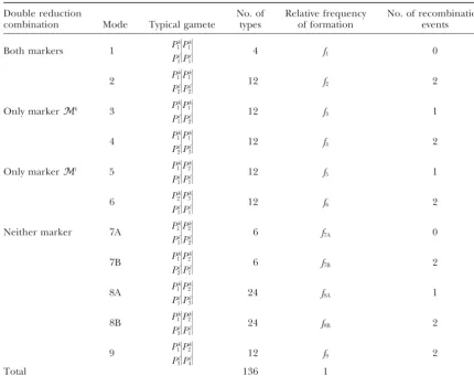
TABLE 1

The model of quadrivalent formation for a diploid gamete in a tetrasomic parent with two linked markersMk_andMl

Double reduction No. of Relative frequency No. of recombination

combination Mode Typical gamete types of formation events

Both markers 1 P

k 1

Pl 1

兩

Pk 1

Pl 1

兩

4 f1 0

2 P

k 1

Pl 2

兩

Pk 1

Pl 2

兩

12 f2 2

Only markerMk ₃ P1k

Pl 1

兩

Pk 1

Pl 2

兩

12 f3 1

4 P

k 1

Pl 2

兩

Pk 1

Pl 3

Pl 4

兩

. _Pk

1, Pk2, Pk3, and Pk4. Given such a fixed assignment for

markerMk_{, we randomly assign the four observed alleles}

of marker Ml_, _Pl

1, Pl2, Pl3, and Pl4, with a total of 24

(5)

different possibilities. One of the possibilities should Pk 1 Pl 1

兩

Pk 2 Pl 2

兩

and P k 1 Pl 2

兩

Pk 2 Pl 1

兩

present a correct assignment for the alleles of the two markers among the four homologous chromosomes.

The estimates of the frequencies of double reduction _{are two reciprocal assignments, but they have the same} and the recombination fraction between the two mark- _{genotype and are mixed in the same cell at row 5 and} ers should be based on their best, but unknown, allelic _{column 5.}

assignment across the parental chromosomes. For link- _{Because formation mode 7 is a mixture of double} age analysis in autotetraploid populations, therefore, a _{recombinants and nonrecombinants, the} determina-vector of unknown parameters can be denoted by␲␻⫽ tion of the expected number of recombination events (A␻, ␣, ␤, ␪)T, where A␻ is the ␻th allelic assignment _{under this mode requires information about the relative}

for marker Ml _{relative to the fixed allelic assignment}

proportions of these two types of offspring. Given the of markerMk_.

relative proportion of double recombinants in mode 7 Given a particular allelic assignment for parent Pas ₍_φ _⫽ _f

7B/f7, see appendix), the expected number of

shown in expression (1), four double reduction gametes _{recombination events is 2}_φ_{. Similarly, for mode 8, which} and six nondouble reduction gametes generated by _{is a mixture of single recombinants and double} recombi-marker Mk _{can be arrayed in the order {}_Pk

1Pk1,Pk2Pk2, _{nants, the expected number of recombination events is}

Pk

3Pk3,Pk4Pk4,Pk1Pk2,Pk1Pk3,Pk1Pk4,Pk2Pk3,Pk2Pk4,P3kPk4} and {Pl1P1l,Pl2Pl2, _{calculated as 1 · (1}⫺ ␺₎⫹_{2 ·}␺ ⫽₁⫹ ␺_{, where} ␺_is

Pl

3Pl3,Pl4Pl4,P1l Pl2,Pl1Pl3,Pl1Pl4,Pl2Pl3,Pl2Pl4,Pl3Pl4} at markerMl. _{the proportion of double recombinants in mode 8}

Thus, we can identify 10⫻10⫽100 two-marker gamete

(␺ ⫽ f8B/f8; seeappendix). The expected numbers of

genotypes for parentP. Following notation inFisher

recombination events between the two markers can be (1947), we definef, the relative frequencies of the 11

expressed in matrix notation as different modes of gamete formation, which must sum

to unity (Table 1). However, because the marker pheno- _D_⫽_{_Dr₁r₂ s₁s₂}10⫻10

types of 7A and 7B cannot be distinguished, we use a singlef7to denote the mixed frequency with which both

7A and 7B occur at meiosis. For the same reason, the mixed frequency of 8A and 8B is denoted byf8. It is not

difficult to express the joint relative frequencies of two-marker diploid gametes in matrix notation:

H⫽{Hr₁r₂

s₁s₂}10⫻10

⫽

Pl

1Pl1

Pl

2Pl2

Pl

3Pl3

Pl

4Pl4

Pl

1Pl2/Pl2Pl1

Pl

1Pl3/Pl3Pl1

Pl

1Pl4/Pl4Pl1

Pl

2Pl3/Pl3Pl2

Pl

2Pl4/Pl4Pl2

Pl

3Pl4/Pl4Pl3







Pk

1Pk1Pk2Pk2Pk3Pk3Pk4Pk4 Pk1Pk2 Pk1Pk3 Pk1Pk4 Pk2Pk3 Pk2Pk4 Pk3Pk4

0 2 2 2 1 1 1 2 2 2

2 0 2 2 1 2 2 1 1 2

2 2 0 2 2 1 2 1 2 1

2 2 2 0 2 2 1 2 1 1

1 1 2 2 2φ 1⫹ ␺1⫹ ␺1⫹ ␺1⫹ ␺ 2

1 2 1 2 1⫹ ␺ 2φ 1⫹ ␺1⫹ ␺ 2 1⫹ ␺

1 2 2 1 1⫹ ␺1⫹ ␺ 2φ 2 1⫹ ␺1⫹ ␺

2 1 1 2 1⫹ ␺1⫹ ␺ 2 2φ 1⫹ ␺1⫹ ␺

2 1 2 1 1⫹ ␺ 2 1⫹ ␺1⫹ ␺ 2φ 1⫹ ␺

2 2 1 1 2 1⫹ ␺1⫹ ␺1⫹ ␺1⫹ ␺ 2φ







.

The above information allows us to express the

recom-⫽

Pl

1Pl1

Pl

2Pl2

Pl

3Pl3

Pl

4Pl4

Pl

1Pl2/Pl2Pl1

Pl

1Pl3/Pl3Pl1

Pl

1Pl4/Pl4Pl1

Pl

2Pl3/Pl3Pl2

Pl

2Pl4/Pl4Pl2

Pl

3Pl4/Pl4Pl3







Pk

1Pk1Pk2Pk2Pk3Pk3Pk4Pk4Pk1Pk2Pk1Pk3Pk1Pk4Pk2Pk3Pk2Pk4Pk3Pk4 1_⁄

4f1 1⁄12f2 1⁄12f2 1⁄12f2 1⁄12f5 1⁄12f5 1⁄12f5 1⁄12f6 1⁄12f6 1⁄12f6 1_⁄

12f2 1⁄4f1 1⁄12f2 1⁄12f2 1⁄12f5 1⁄12f6 1⁄12f6 1⁄12f5 1⁄12f5 1⁄12f6 1_⁄

12f2 1⁄12f2 1⁄4f1 1⁄12f2 1⁄12f6 1⁄12f5 1⁄12f6 1⁄12f5 1⁄12f6 1⁄12f5 1_⁄

12f2 1⁄12f2 1⁄12f2 1⁄4f1 1⁄12f6 1⁄12f6 1⁄12f5 1⁄12f6 1⁄12f5 1⁄12f5

1_⁄

12f3 1⁄12f3 1⁄12f4 1⁄12f4 1⁄6f7 1⁄24f8 1⁄24f8 1⁄24f8 1⁄24f8 1⁄6f9 1_⁄

12f3 1⁄12f4 1⁄12f3 1⁄12f4 1⁄24f8 1⁄6f7 1⁄24f8 1⁄24f8 1⁄6f9 1⁄24f8 1_⁄

12f3 1⁄12f4 1⁄12f4 1⁄12f3 1⁄24f8 1⁄24f8 1⁄6f7 1⁄6f9 1⁄24f8 1⁄24f8 1_⁄

12f4 1⁄12f3 1⁄12f3 1⁄12f4 1⁄24f8 1⁄24f8 1⁄6f9 1⁄6f7 1⁄24f8 1⁄24f8 1_⁄

12f4 1⁄12f3 1⁄12f4 1⁄12f3 1⁄24f8 1⁄6f9 1⁄24f8 1⁄24f8 1⁄6f7 1⁄24f8 1_⁄

12f4 1⁄12f4 1⁄12f3 1⁄12f3 1⁄6f9 1⁄24f8 1⁄24f8 1⁄24f8 1⁄24f8 1⁄6f7







. bination fraction␪and the two double reduction param-eters,␣at markerMk_and␤_{at marker}Ml_{, in terms of} f1, . . . ,f9andφ,␺. We have

␣ ⫽f1⫹f2⫹f3⫹f4;

␤ ⫽f1⫹f2⫹f5⫹f6;

2␪ ⫽(f3⫹f5)⫹2(f2⫹f4⫹f6⫹f9)⫹2φf7⫹(1⫹ ␺)f8.

(2)

From the above equations, it follows that |␣ ⫺ ␤|⫽|f3⫹

However, as illustrated earlier, there are as many as 136

f4 ⫺ f5 ⫺ f6) ⱕ f3 ⫹ f4 ⫹ f5 ⫹ f6 ⱕ 2␪. Therefore the

gamete formations for any two linked markers. The 36

difference in the frequency of double reduction be-“extra” gamete formations are each due to a reciprocal

tween two loci is bounded by two times the recombina-allelic assignment of markerMl_{and are located in the}

tion fraction in tetraploid. This inequality is consistent 6 ⫻ 6 ⫽ 36 cells of the above matrix’s bottom-right

with the fact that when two markers are close, their corner, in which neither of the two markers displays

double reduction rates tend to be similar. We believe double reduction (Table 1). Of these 36 formations, 6

similar inequalities exist for other ploidy levels. How-are under mode 7, 24 How-are under mode 8, and the

re-ever, due to complexity of gamete types for those cases, maining 6 are under mode 9. For example, gamete

(6)

For a fully informative marker, every gamete genotype

␪ ⫽ 1

2N[N3⫹N5⫹2(N2⫹ N4⫹ N6⫹ N9) can be well distinguished. Thus, N offspring in a

full-sib family can be sorted into the nine distinguishable

gamete formation modes of sizeN1,N2, . . . ,N9, respec- ⫹ 2␪ 2

2␪2⫺₁₈␪ ⫹₉N7⫹

3⫺ ␪

3⫺2␪N8]. (6) tively (see Table 1). It is not difficult to derive the

ex-plicit expressions of the maximum-likelihood estimates _{Since this a fourth-order polynomial of}_␪_{, closed-form} for the frequencies of these nine formation modes f1, _{solutions exist and can be calculated very easily.}

f2, . . . ,f9in terms of the corresponding sample frequen- _{The characterization of linkage phase:} _{We derived}

ciesN1,N2, . . . ,N9on the basis of the following likelihood _{statistical procedures for estimating} ␣_, ␤_{, and} ␪ _when

function given the observed marker data (M): _{the allelic assignment as shown in expression (1) is} assumed. The estimates of parameters (␣,␤,␪) for any

ᐉ(f|M)⫽

冢

N

N1 . . .N9冣

兿

9

i⫽1

fN_i

i . one of the other 23 assignments can be similarly

ob-tained by changing the positions of the corresponding elements in matricesHandD. One remaining issue is From the above matrixH, which indicates where double

how to determine the best assignment,i.e., one corre-reduction has occurred for each of the markers, the

sponding to a most likely parental linkage phase of two double-reduction parameters,␣and␤, can be

esti-the two markers. The most likely linkage phase can be mated in terms of the corresponding frequencies of

determined using the posterior probability of␲␻⫽(A␻, formation modes;i.e.,␣ˆ ⫽(N1⫹N2⫹N3⫹N4)/Nand

␣,␤,␪)T_{conditional on the marker data}_M_{, where}_A

␻

␤ˆ _⫽ ₍_N₁ _⫹ _N₂ _⫹ _N₅ _⫹ _N₆_)/_N_{. Since these are simply}

is the␻th allelic assignment for markerMl_{relative to}

estimates of binomial proportions, the variances of ␣ˆ

the fixed allelic assignment of markerMk_{. From Bayes’}

and␤ˆ are␣(1⫺ ␣)/N and␤(1⫺ ␤)/N, respectively.

theorem: Suppose we could distinguish the twof7modes and

the twof8modes; the likelihood function given complete

P(␲␻|M)⫽ P(␲␻)P(M|␲␻)

R24

␻⫽1P(␲␻)P(M|␲␻)

. data (N1,N2, . . . ,N6,N7A,N7B,N8A,N8B,N9) is

These posterior probabilities for all possible

assign-ᐉ(f|M)⫽

冢

N

N1. . .N9冣冢

兿

6

i⫽1

fN_i

i

冣

fN_7A7AfN_7B7Bf_8AN8AfN_8B8BfN99. (3)

ments depend on the prior probabilitiesP(␲␻). In prac-tice, the prior distribution can be assumed to be uniform On the basis of the observed incomplete dataN1,N2, . . . ,

among all 24 assignments and, in this case, the posterior N7, N8, N9, the EM algorithm is used to estimate the

probabilities are proportional to the likelihoods recombination fraction by maximizing the likelihood

L(␲␻)⫽ P(M|␲␻). The final MLEs for the parameters Equation 3 (Dempsteret al.1977;LanderandGreen

(␣,␤,␪) are based on the most likely assignment with 1987). The general equations formulating the iteration

the highest posterior probability. of the␶ ⫹1)th EM step are given as follows:

Sved (1964) demonstrated that, unless they solely E step: Calculate the expected number of recombina- form bivalents, autotetraploids have a recombination

tion events between markers Mk_andMl_{for all}

off-fraction bounded by 1 ⫺ 1/x, where x is the level of spring with no occurrence of double reduction. This ploidy. Thus, for autotetraploids undergoing quadriva-is equivalent to estimating φ for mode 7 and ␺ for lent pairings, the maximum value of recombination mode 8, respectively, by fraction is␪ ⫽0.75. The test of whether or not the two given markers are linked is based on the log-likelihood-ratio test statistic under the full model (Equation 3), φˆ(␶)⫽ [␪(␶)]2

2[␪(␶)_]2⫺₁₈␪(␶)⫹₉, ␺ˆ

(␶)⫽ ␪(␶)

3⫺2␪(␶). (4)

which corresponds to the parameter estimators derived from the most likely assignments, and the reduced M step: Maximize the expected log-likelihood of ␪.

model with the restraint of␪ ⫽ 0.75. The likelihood-This gives an updated estimate for the recombination

ratio test (LRT) statistic calculated in this way has a

fraction and is obtained as _␹₂

-distribution with1_⁄

2 d.f. under the null hypothesis

(SelfandLiang1987). Thus, two markersMk_andMl

␪ˆ(␶⫹1)⫽ 1

2N[N3 ⫹N5 ⫹2(N2⫹N4⫹N6⫹N9) can be declared to be linked if the LRT is ⬎ ␹21/2,␦for

an appropriate choice of the type I error rate ␦ (for

⫹2φˆ(␶)_N

7⫹(1⫹ ␺ˆ(␶))N8]. (5) _example,␹2_1/2,0.05⫽_2.42).

These two steps are repeated until the estimate of␪

converges to a stable value. Such a stable value is the SIMULATION maximum-likelihood estimate (MLE) of␪.

Analysis of a simulated data set: We illustrate the autotetraploid model through analyzing a simulated ex-If we plugφand␺from Equations 4 into 5, we can

(7)

we consider analysis only on the segregation of the ga- Pk 1

Pl 1

兩

Pk 3

Pl 4

兩

mete genotypes in parentP, which is assumed to have frequencies of double reduction (0.05, 0.1) and

recom-bination fraction 0.05. These parameters correspond to should be in mode 7 instead of mode 8. The counts for all nine gamete formation modes, under the new relative frequencies of the nine different gamete

forma-tion modes f ⫽ (0.04071, 0.00130, 0.00446, 0.00353, assignments, areN1 ⫽7,N2⫽7,N3⫽ 2,N4⫽1,N5⫽

5,N6⫽5,N7⫽53,N8⫽123,N9⫽0. Consequently, we

0.04301, 0.01498, 0.88221, 0.00736, 0.00245), which give

the joint relative frequencies of two-marker diploid ga- can obtain the MLE (␣ˆ,␤ˆ,␪ˆ)⫽ (0.07, 0.105, 0.46436) with log-likelihood llA ⫽ ⫺758.50. Similar to the first

metes in the matrixH. A random sample of N ⫽200

gametes was simulated from multinomial distribution assignment, we also have MLE (␣ˆ,␤ˆ,␪ˆ)⫽(0.118, 0.208, 0.75) with log-likelihood llN⫽ ⫺786.47 under the null

with probabilities given byH.The marker dataM,e.g.,

the counts of all gamete types, can be presented in the hypothesis.

This procedure needs to be repeated for all of the following matrix form:

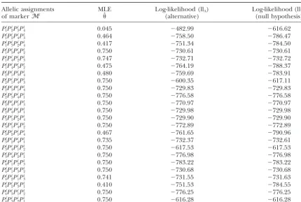
other 22 assignments. In Table 2, we present MLEs and log-likelihood for all 24 different allelic assignments. Figure 2 (top left) plotted the log-likelihood values against the 24 assignments of markerMl_{with a}

diction-ary order 1234, 1243, . . . , 4321. Estimates of the recom-bination fraction for different assignments are indicated by different insets in the figure. It shows that a true assignment has the largest log-likelihood value. Pl

1Pl1

Pl 2Pl2

Pl 3Pl3

Pl 4Pl4

Pl 1Pl2/Pl2Pl1

Pl 1Pl3/Pl3Pl1

Pl 1Pl4/Pl4Pl1

Pl 2Pl3/Pl3Pl2

Pl 2Pl4/Pl4Pl2

Pl 3Pl4/Pl4Pl3







Pk

1Pk1Pk2Pk2Pk3Pk3Pk4Pk4Pk1Pk2Pk1Pk3Pk1Pk4Pk2Pk3Pk2Pk4Pk3Pk4

3 0 0 0 1 2 0 0 0 0

0 4 0 0 1 0 0 1 0 0

0 0 3 0 1 0 0 1 0 0

0 0 0 1 0 0 1 0 2 0

0 2 0 0 22 0 1 0 0 0

0 0 0 0 0 16 0 0 0 0

0 0 0 0 0 0 33 1 0 0

0 0 0 0 1 0 0 35 0 0

0 0 0 1 0 0 0 0 36 0

0 0 0 0 0 0 0 0 0 31







.

Since assignment 1 has the largest log-likelihood, we choose the final MLEs for the parameters on the basis of the first assignment; e.g., (␣ˆ, ␤ˆ, ␪ˆ) ⫽ (0.07, 0.105, 0.453) with log-likelihood llA⫽ ⫺482.98. However,

un-der the null hypothesis, the final MLE comes from the last assignment with log-likelihood llN⫽ ⫺616.28. Thus

the LRT statistic equals⫺2 ⫻ (⫺616.28⫹ 482.98) ⫽ Suppose parentP has alignment 266.60, which is much larger than the cut point value

␹2

1/2,0.05⫽2.42, implying that there is very strong

evi-dence that the two markers are linked. Pk

1

Pl 1

兩

Pk 2

Pl 2

兩

Pk 3

Pl 3

兩

Pk 4

Pl 4

兩

;

More simulations: Extensive simulation studies were performed to investigate the properties of our statistical then there are 11 offspring in the first gamete formation _{method by evaluating the effectiveness of determining} mode (N1⫽3⫹ 4⫹ 3⫹ 1). Similarly, counts for the _{a correct allelic assignment, the precision of the}

parame-other eight modes areN2⫽0,N3⫽3,N4⫽0,N5⫽9, _{ter estimates, and the power to detect linkage. A number}

N6⫽1,N7⫽ 173,N8⫽ 2, andN9⫽ 1. Hence we have _{of genetic scenarios are designed to explore the effects}

MLEs of the relative frequencies of the nine different

of different parameter values on their estimation from gamete formation modes fˆ ⫽ (11/200, 0, 3/200, 0,

this new method. A segregating full-sib family of size 9/200, 1/200, 173/200, 2/200, 1/200), which

corre-N⫽80, 200, 400, or 800 is simulated by hypothesizing spond to␣ˆ⫽(N1⫹N2⫹N3⫹N4)/N⫽0.07,␤ˆ⫽(N1⫹ _{different recombination fractions ranging from tight}

N2 ⫹ N5 ⫹ N6)/N ⫽ 0.105, and␪ˆ ⫽ 0.0453 with log- _{linkage to free recombination,}_{␪ ⫽}_{0.05, 0.15, 0.25, 0.50,}

likelihood (ll)A⫽ ⫺482.98. Furthermore, under the null _{0.65, and 0.75, and different pairs of double reduction}

hypothesis␪ ⫽0.75, the MLEs of mode frequencies are _{rates with various degrees of difference between two} fˆ⫽(0.01396, 0, 0.00757, 0, 0.02272, 0.25448, 0.43679, _{markers, (}_␣_, _␤₎_⫽ _{(0.05, 0.1), (0.15, 0.2), (0.25, 0.3),} 0.01, 0.25448), and the parameter estimates are ␣ˆ ⫽ _{(0.1, 0.2) and (0.05, 0.3). For}_{␪ ⫽}_{0.05, however, only} 0.022,␤ˆ ⫽ 0.291 with llN⫽ ⫺616.62. _{the first three pairs of (}␣_, ␤_{) are considered because}

For a second assignment _{the other two combinations are impossible (recall |}_{␣ ⫺}

␤|ⱕ2␪). The simulation is repeated 1000 times for each Pk

Pk 3

Pl

4

兩

In Figure 2, the log-likelihood values are plotted

against the 24 different allelic assignments of marker has no recombination and should be classified into Ml_{with a dictionary order 1234, 1243, . . . , 4321. For}

(8)

TABLE 2

Maximum-likelihood estimates␪ˆ of the recombination fraction with all 24 different allelic assignments of markerMl_{for the simulated example}

Allelic assignments MLE Log-likelihood (llA) Log-likelihood (llN)

of markerMl ␪_ˆ _{(alternative)} _{(null hypothesis)}

Pl

1Pl2Pl3Pl4 0.045 ⫺482.99 ⫺616.62

Pl

1Pl2Pl4Pl3 0.464 ⫺758.50 ⫺786.47

Pl

1Pl3Pl2Pl4 0.417 ⫺751.34 ⫺784.50

Pl

1Pl3Pl4Pl2 0.750 ⫺730.61 ⫺730.61

Pl

1Pl4Pl2Pl3 0.747 ⫺732.71 ⫺732.72

Pl

1Pl4Pl3Pl2 0.475 ⫺764.19 ⫺788.37

Pl

2Pl1Pl3Pl4 0.480 ⫺759.69 ⫺783.91

Pl

2Pl1Pl4Pl3 0.750 ⫺600.35 ⫺617.11

Pl

2Pl3Pl1Pl4 0.750 ⫺729.83 ⫺729.83

Pl

2Pl3Pl4Pl1 0.750 ⫺776.58 ⫺776.58

Pl

2Pl4Pl1Pl3 0.750 ⫺770.97 ⫺770.97

Pl

2Pl4Pl3Pl1 0.750 ⫺729.98 ⫺729.98

Pl

3Pl1Pl2Pl4 0.750 ⫺729.90 ⫺729.90

Pl

3Pl1Pl4Pl2 0.750 ⫺772.89 ⫺772.89

Pl

3Pl2Pl1Pl4 0.467 ⫺761.65 ⫺790.96

Pl

3Pl2Pl4Pl1 0.735 ⫺732.37 ⫺732.61

Pl

3Pl4Pl1Pl2 0.750 ⫺617.53 ⫺617.53

Pl

3Pl4Pl2Pl1 0.750 ⫺776.98 ⫺776.98

Pl

4Pl1Pl2Pl3 0.750 ⫺783.22 ⫺783.22

Pl

4Pl1Pl3Pl2 0.750 ⫺730.68 ⫺730.68

Pl

4Pl2Pl1Pl3 0.741 ⫺731.55 ⫺731.63

Pl

4Pl2Pl3Pl1 0.410 ⫺751.53 ⫺784.55

Pl

4Pl3Pl1Pl2 0.750 ⫺776.25 ⫺776.25

Pl

4Pl3Pl2Pl1 0.750 ⫺616.28 ⫺616.28

The last two columns are the log-likelihood (llA) under alternative hypothesis and (llN) under null hypothesis

(␪ ⫽0.75).

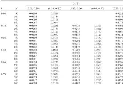
bination fraction are obtained, as indicated by different depends on true double reduction rates (␣,␤) with two tendencies (Table 3). First, the RMSEs tend to be larger insets in the figure. It is shown that a true assignment

usually corresponds to the largest log-likelihood value. when there are larger double reduction rates. Second, the RMSEs tend to increase when the difference of There is a distinct difference between the largest and

the second-largest log-likelihood values, especially when double reduction between the two markers increases. For example, the RMSEs of␪ˆ⫽0.5 or above are larger

␪is small. This implies that our method can well be used

to characterize the marker linkage phase in parents. In for (␣,␤)⫽(0.10, 0.20) than (0.25, 0.30), although the latter combination has larger double reduction rates. some cases, the second-largest log-likelihood value is

The power to detect a significant linkage is examined associated with the estimate of␪ ⬎0.75, so it is easy to

on the basis of 1000 replicates (Figure 3). Obviously, avoid the assignment corresponding to such an

esti-the power of esti-the test increases with increasing sample mate.

sizes. However, the effect of sample size depends on the We did not report simulation results about double

double reduction rates and recombination fraction. For reduction rate estimates␣ˆ and␤ˆ because we have

closed-example, the effect is larger for (␣,␤)⫽(0.1, 0.2) than form formulas for their variances. To evaluate the

preci-for (␣, ␤) ⫽ (0.15, 0.2) when ␪ ⫽ 0.65, but this is sion of the recombination fraction estimates,

square-reversed for␪ ⫽0.5. rooted mean square errors (RMSEs) are calculated for

all simulation scenarios (Table 3). As expected, the RMSEs decrease with increasing sample sizes. However,

DISCUSSION sample size effects also decrease with increasing sample

(9)

Figure

2.—Plot

of

the

log-likelihood

(ll)

vs.

24

assignments

for

18

sets

of

parameters

(

␪

,

␣

,

␤

)

from

one

simulation

with

sample

size

N

⫽

200.

The

x

-axes

are

the

24

assignments

in

d

ictionary

order,

i.e.

,

1

234,

1243,

.

,

4321.

D

ifferent

symbols

used

in

the

plots

indicate

the

range

of

MLE

␪

ˆfor

e

ach

assignment:

circles

for

␪

ˆin

(0,

1/8];

crosses

for

(1/8,

3/8];

stars

for

(3/8,

5/8];

diamonds

for

(5/8,

3/4];

and

squares

for

o

thers.

The

MLE

␪

ˆ ’s

corresponding

to

the

m

ost

likely

assignment

are

indicated

in

each

(10)

TABLE 3

Square-rooted mean square error (RMSE) for the estimator␪ˆ of the recombination fraction for all 28 combinations of parameters (␪,␣,␤) and four sample sizesN

(␣,␤)

␪ N (0.05, 0.10) (0.10, 0.20) (0.15, 0.20) (0.05, 0.30) (0.25, 0.30)

0.05 80 0.0209 0.0236 0.0222

200 0.0132 0.0144 0.0142

400 0.0090 0.0101 0.0100

800 0.0067 0.0074 0.0073

0.15 80 0.0408 0.0281 0.0375 0.0370 0.0364

200 0.0265 0.0180 0.0245 0.0242 0.0300

400 0.0183 0.0129 0.0173 0.0167 0.0161

800 0.0130 0.0087 0.0118 0.0121 0.0112

0.25 80 0.0439 0.0465 0.0471 0.0487 0.0491

200 0.0301 0.0297 0.0292 0.0321 0.0311

400 0.0203 0.0203 0.0211 0.0226 0.0219

800 0.0138 0.0145 0.0149 0.0153 0.0157

0.50 80 0.0793 0.1051 0.1220 0.0904 0.1076

200 0.0396 0.0482 0.0508 0.0481 0.0471

400 0.0267 0.0291 0.0304 0.0331 0.0296

800 0.0201 0.0217 0.0206 0.0234 0.0197

0.65 80 0.0853 0.0733 0.0685 0.0879 0.0535

200 0.0726 0.0492 0.0462 0.0669 0.0366

400 0.0573 0.0351 0.0340 0.0554 0.0259

800 0.0361 0.0258 0.0243 0.0414 0.0187

0.75 80 0.0435 0.0634 0.0528 0.0664 0.0341

200 0.0223 0.0329 0.0230 0.0402 0.0227

400 0.0142 0.0219 0.0143 0.0285 0.0153

800 0.0098 0.0126 0.0107 0.0221 0.0115

ysis in autopolyploids, many earlier methods assume a bounded by two times their recombination fraction in tetraploid.

pure bivalent pairing model between homologous

chro-mosomes during meiosis (Wuet al.1992; Hackett et With these underpinning mechanisms of quadriva-lent pairings, Fisher (1947) formulated a pioneering al.1998;Ripolet al.1999;Luoet al.2001). Although the

statistical merits of these methods were demonstrated by genetic model to count all possible modes of gamete formation in autotetraploids. But, in his time, he could extensive simulations, their underlying assumption may

significantly deviate from biological reality. For an auto- not separate and further estimate two different modes generating the same gamete genotypes (e.g., mode 7A polyploid, multivalent pairings during gametogenesis

may result in double reduction (Darlington1929;de vs. 7B or mode 8A vs. 8B; Table 1). Thanks to the development of the maximum-likelihood method

im-Winton and Haldane 1931; Mather 1936; Fisher

1947), a phenomenon that adds extra complexity in plemented with the EM algorithm (Dempster et al. 1977), we are now able to well discriminate and estimate the establishment of a workable model for polysomic

linkage analysis. the proportions of these different modes by viewing

them as a missing data problem. In this article, we derive a statistical method for

simul-taneously estimating the linkage and linkage phase be- The advantage of the EM algorithm is that it resulted in closed-form solution for the recombination fraction. tween different markers in a full-sib family of

autotetra-ploids undergoing quadrivalent pairings at meiosis. This However, if we forego this, it is also possible to perform a Bayesian analysis. We may assign a Dirichlet prior for method based on quadrivalent pairings is not a simple

extension of the existing models on bivalent pairing. the frequencies of the nine formation modesf⫽(f1,f2,

. . . ,f9), which yields a Dirichlet posterior distribution

Rather, the method has incorporated the cytological

mechanisms underlying gamete formation derived from offgiven the sample frequenciesN1,N2, . . . ,N9. Thus

we can easily sample from the posterior offand obtain multivalent pairings, some of which (i.e., double

reduc-tion) are unique and do not happen with bivalent pair- a posterior sample of (␣,␤,␪) by letting␣ ⫽f1⫹f2⫹

f3⫹f4,␤ ⫽f1⫹f2⫹f5⫹f6and solving␪using Equation

ings. We also showed that the difference in the

(11)

Figure 3.—The size and power of the likelihood-ratio test of linkage using␹2

1/2,0.05⫽

2.42 on the basis of 1000 repli-cates. The power (or size) of the test vs. true ␪ for all five sets of double reduction rates was plotted.

this to the 11 basic gamete modesf*⫽(f1,f2, . . . ,f6, gote genotypes, because the segregation at the gamete

level cannot provide adequate information for linkage f7A, f7B, f8A, f8B, f9), then a Gibbs sampler could be set

up to obtain posterior samples (Robert andCasella analysis.

Second, our method is based on a single pairing 2000).

Although we have devised a statistical method for model—quadrivalent. Chromosome pairings in auto-polyploids indeed are a function of the homology resolving a fundamentally important problem in

auto-polyploid linkage analysis, one that has puzzled geneti- between the genomes involved, with a propensity in pairing between homologous over homeologous chromo-cists for over one-half century, there is still much room

for improvement. First, our model is proposed for fully somes, which is defined as the preferential pairing factor (Sybenga1994). Such a preferential pairing factor de-informative codominant markers,i.e., those of eight

dif-ferent alleles between the two autotetraploid parents at termines the relative importance of bivalentvs. multiva-lent pairings in autopolyploids and, therefore, can be each marker. For these markers, an explicit expression

exists for the MLE of the frequency of double reduction, used to model the frequency of double reduction and recombination fraction when both bivalent and multiva-although the estimate of the recombination fraction

must rely upon EM iterations. In a practical full-sib map- lent pairings happen simultaneously during meiosis. Last, our method is developed for autotetraploids, but ping population, other types of markers, such as

domi-nant or partially informative, may be common. For auto- its extension to autohexaploid, autooctoploid, and auto-dexaploid species is important because many important polyploids, dominant markers derived from randomly

amplified polymorphic DNA or amplified fragment plant species have such high ploidy levels (Soltisand

Soltis2000). For an autohexaploid plant, for instance,

length polymorphism technologies typically cannot be

distinguished among simplex (single dose), duplex triploid gametes are generated at meiosis, including three gamete types of pure double reduction, partial (double dose), and multiplex (multiple dose) types,

because they present an identical genotype (Wuet al. double reduction, and no double reduction.

The statistical method proposed in this article de-1992;Yu andPauls 1993;Luo et al. 2000). For these

dominant or partially informative markers, gametes scribes a mapping framework for studying the genome structure and organization in complex autopolyploid formed with double reduction may have the same

geno-types as those formed without double reduction. Thus, species, providing a sophisticated model for linkage analysis in autopolyploids. It provides a necessary plat-estimating the frequency of double reduction will have

(12)

zy-Masterson, J., 1994 Stomatal size in fossil plants—evidence for important traits in autopolyploids. Although some

pre-polyploidy in majority of angiosperms. Science264:421–424. liminary studies have been reported for QTL mapping _{Mather, K.,} ₁₉₃₆ _{Segregation and linkage in autotetraploids. J.}

Genet.32:287–314. in autopolyploids, assuming pure bivalent pairings

Meyer, R. C., D. Milbourne, C. A. Hackett, J. E. Bradshaw, J. W. (DoergeandCraig2000;XieandXu2000), all of these

McNicholandR. Waugh,1998 Linkage analysis in tetraploid should be viewed as premature until a comprehensive _{potato and association of markers with quantitative resistance to} late blight (Phytophthora infestans). Mol. Gen. Genet.259:150–160. model is framed to take both bivalent and multivalent

Otto, S. P.,andJ. Whitton,2000 Polyploid incidence and evolu-pairings into account.

tion. Annu. Rev. Genet.34:401–437.

Ripol, M. I., G. A. Churchill, J. A. G. da SilvaandM. Sorrells, We are grateful to Dr. S. Xu and Dr. M. Gallo-Meagher for

stimulat-1999 Statistical aspects of genetic mapping in autopolyploids. ing discussions regarding this project. The authors thank the associate

Gene235:31–41. editor, referee Dr. R. Deborah Overath, and one anonymous referee

Robert, P. C.,andG. Casella,2000 Monte Carlo Statistical Methods for their constructive comments. This manuscript was approved as

(Springer Texts in Statistics). Springer-Verlag, New York. Journal Series R-08464 by the Florida Agricultural Experiment Station.

Self, S. G.,andK. Y. Liang,1987 Asymptotic properties of maximum likelihood estimators and likelihood ratio tests under nonstan-dard condition. J. Am. Stat. Assoc.82:605–610.

Soltis, P. S.,andD. E. Soltis,2000 The role of genetic and genomic LITERATURE CITED _{attributes in the success of polyploids. Proc. Natl. Acad. Sci. USA}

97:7051–7057. Bever, J. D.,andF. Felber,1992 The theoretical population

genet-Stebbins, G. L.,1971 Chromosomal Evolution in Higher Plants. Addi-ics of autopolyploidy. Oxf. Surv. Evol. Biol.8:185–217.

son-Wesley, Reading, MA. Brouwer, D. J.,andT. C. Osborn,1999 A molecular marker linkage

Sved, J. A.,1964 The relationship between diploid and tetraploid map of tetraploid alfalfa (Medicago sativaL.). Theor. Appl. Genet.

recombination frequencies. Heredity19:585–596. 99:1194–1200.

Sybenga, A.,1994 Preferential pairing estimates from multivalent Darlington, C. D.,1929 Chromosome behaviour and structural

frequencies in tetraploids. Genome37:1045–1055. hybridity in the Tradescantiae. J. Genet.21:207–286.

Wu, K. K., W. Burnquist, M. E. Sorrells, T. L. Tew, P. H. Moore da Silva, J., M. E. Sorrells, W. L. BurnquistandS. D. Tanksley, _{et al., 1992} _{The detection and estimation of linkage in polyploids}

1993 RFLP linkage map and genome analysis ofSaccharum

spon-using single-dose restriction fragments. Theor. Appl. Genet.83: taneum.Genome36:782–791.

L294–300. Dempster, A. P., N. M. LairdandD. B. Rubin,1977 Maximum

Xie, C. G.,andS. H. Xu,2000 Mapping quantitative trait loci in likelihood from incomplete data via EM algorithm. J. Stat. Soc.

tetraploid populations. Genet. Res.76:105–115.

Ser. B39:1–38. _{Yu, K. F.,}_and_{K. P. Pauls,}₁₉₉₃ _{Segregation of random amplified} de Winton, D.,andJ. B. S. Haldane,1931 Linkage in the tetraploid _{polymorphic DNA markers and strategies for molecular mapping}

Primula sinensis.J. Genet.24:121–144. _{in tetraploid alfalfa. Genome}_36:_844–851. Doerge, R. W.,andB. A. Craig,2000 Model selection for

quantita-tive trait locus analysis in polyploids. Proc. Natl. Acad. Sci. USA Communicating editor:J. B. Walsh 97:7951–7956.

Fisher, R. A.,1947 The theory of linkage in polysomic inheritance. Philos. Trans. R. Soc. Ser. B233:55–87.

APPENDIX Grant, V.,1981 Plant Speciation, Ed. 2. Columbia University Press,

New York.

Among the 16 possible allele configurations, 4 have Grivet, L., A. D’Hont, D. Roques, P. Feldmann, C. Lanaudet al.,

no recombination and 12 have one recombination. If 1996 RFLP mapping in cultivated sugarcane (Saccharum spp):

genome organization in a highly polyploid and aneuploid inter- _{we form gametes with two chromosomes by selecting,} specific hybrid. Genetics142:987–1000. _{with replacement, from the 16 alleles twice, this yields} Hackett, C. A., J. E. Bradshaw, R. C. Meyer, J. W. McNicol, D.

16⫻16⫽256 possibilities (16 with no recombination, Milbourneet al., 1998 Linkage analysis in tetraploid species:

a simulation study. Genet. Res.71:143–154. _{96 with one recombination, and 144 with two).} Hilu, K. W.,1993 Polyploidy and the evolution of domesticated _{Recall that} _φ _and _␺ _{are the proportions of gamete}

plants. Am. J. Bot.80:1491–1499.

types that have two recombination events under modes Jackson, R. C.,andJ. W. Jackson,1996 Gene segregation in

autotet-raploids: prediction from meiotic configurations. Am. J. Bot.83: 7 and 8, respectively. Note that f7A contains 12 out of

673–678. _{16 gametes with no recombination and}_f

7Bcontains 12

Lander, E. S.,andP. Green,1987 Construction of multilocus

ge-out of 144 gametes with two recombinations; thus the netic linkage maps in human. Proc. Natl. Acad. Sci. USA 84:

2363–2367. relative proportions should be 12(1 ⫺ ␪)2_/16:12␪2_/

Luo, Z. W., C. A. Hackett, J. E. Bradshaw, J. W. McNicoland ₁₄₄_⫽ ₉₍₁_{⫺ ␪}₎2_:␪2_{. Similarly,} _f

8Acontains 48 out of 96

D. Milbourne,2000 Predicting parental genotypes and gene

gametes with one recombination and f8B contains 48

segregation for tetrasomic inheritance. Theor. Appl. Genet.100:

1067–1073. out of 144 gametes with two recombinations; thus the

Luo, Z. W., C. A. Hackett, J. E. Bradshaw, J. W. McNicolandD. _{relative proportions should be 48}_⫻₂_␪₍₁_{⫺ ␪}_)/96:48_⫻ Milbourne,2001 Construction of a genetic linkage map in

␪2_/144⫽₃₍₁⫺ ␪_):␪_{. Consequently, we may assume}φ⫽

tetraploid species using molecular markers. Genetics157:1369–