Model Formulation of Drinking Behavior Using Longitudinal Data
H. T. Banks, Keri L. Rehm, Karyn L. Sutton Center for Research in Scientific Computation Center for Quantitative Science in Biomedicine
North Carolina State University Raleigh, NC 27695-8212
and
Christine Davis, Lisa Hail, Alexis Kuerbis, Jon Morgenstern Substance Abuse Services
Department of Psychiatry Columbia University Medical Center
180 Fort Washington Ave. HP-240 NYC, NY 10032
Dec 8, 2010
Abstract
We present a novel dynamical systems modeling approach to an intensive longitudinal data set of inter- and intrapersonal factors in problem drinkers. To our knowledge, there have been no such models developed in this area on the individual level. As a result, considerable effort was required to determine the variables of interest in such a model, possible, if any, relationships between them, and even the timescale on which to observe them. We discuss the construction of an initial mathematical model with the potential to help in understanding the underlying mechanisms responsible for behavior change in problem drinkers.
1
Introduction
In the field of drug and alcohol abuse, many researchers have collected vast amounts of informa-tion on substance use, participant’s willingness to change behavior, and participant’s success in a particular treatment. Using this information, field experts have formulated ideas about difficult-to-measure factors that control a patient’s motivations and behavior, such as salience – the value of drinking in relation to other activities, commitment to a favorable outcome and reduced alcohol consumption, and recognition of reasons to not use a substance. However, the relative contributions of these driving factors as they form mechanisms for behavior change are unclear. The interplay of these factors as they change over time is a natural question to address via a mathematical model, which enables us to describe these processes quantitatively as a dynamical system. We seek to model these ideas of a drinking behavior control system as informed by a dataset, Project MOTION, to gain insight into the underlying mechanisms.
or 56 days, and gave information about inter- and intrapersonal factors that could potentially influence their drinking as well as their drinking behavior in the past 24 hrs and their commitment to avoid heavy drinking or drinking at all in the next day.
There is no straightforward way of organizing data on such a large variety of aspects of daily life into a reasonable number of variables to study within a mathematical modeling framework. Further complicating this issue is the lack of previous modeling efforts in this area, resulting in a lack of pertinent quantities commonly agreed upon. To begin formulating conceptual variables, we applied linear methods such as calculating coefficients of determination, linear interpolation via least-squares approximation and principal component analysis. However, these methods do not provide any useful information on relationships between an individual’s responses to questions. It is sensible to construct our model variables on questions based on similar ideas used in the IVR. We shall examine how these categories relate to each other, and how to best use this data in formulating a model. Our initial interpretation of this data is based on knowledge and predictions from the field of substance abuse and recovery, visually assessing qualitative trends between similar questions within topical categories, and grouping them into variables. Once variables were decided upon, qualitative trends between them were examined to determine the existence and nature of relationships between them within a single patient.
Generally, for mathematical modeling to be effective, it should be done as an iterative process in which an initial model is formulated and then compared with observed or experimental data. This comparison gives insight into any discrepancies between the observed processes and model predictions, suggesting refinements to the model. This process is repeated until the model provides sufficient information to capture key aspects of behavior of the observed system and to answer questions of interest. Our approach, as described in this document, can be briefly outlined as follows: we initiate this iterative process and formulate a mathematical model of differential equations using the newly formed variables from the IVR data set.
We construct this first model based on prior knowledge of hypothesized relationships between the model variables based on knowledge of substance abuse therapy and relationships observed in the data from Project MOTION. We seek to construct a model such that solutions agree with our prior knowledge and are similar to the data. The processes involve nonlinear and delayed components contributing to decision-making and behavior modification mechanisms. This initial model is then compared to data of selected patients, and further refinements and next steps are discussed.
2
Background literature
Many groups have explored the use of various mathematical models and concepts to explain some aspects of drinking behavior and of behavior change. Many mathematical models found in literature are relatively simplistic and focus only on a small number of forces that may influence a person’s or cohort’s behavior patterns, and a number of these models lack comparisons to data. The most popular modeling techniques are based on diffusion through social structures and SIR (Succeptible - Infected - Recovered) models for infectious diseases. Unlike these models, we intend for our proposed dynamical system model to describe individual-level dynamics.
participant’s substance use. These studies provide useful information to be drawn upon in our modeling efforts.
2.1 Mathematical Models in Alcohol Studies
A number of compartmental models have been developed to roughly explain substance use in a cohort. These models generate information regarding long term outcomes in substance use; namely, they attempt to determine the chances a person will become a regular user or even heavy user if he/she starts using a substance with a particular frequency. These models typically do not provide information regarding the changes a person experiences while transitioning from different levels of use and therefore cannot be used to inform reasons for behavior change. Additionally, these models are cohort-centric and may not be applicable to other groups in a population, of different drinking behavior.
In Scribner et al. [72] and Ackleh et al., [2] an ODE compartmental model which classifies students according to drinking habits (abstainers, moderate, etc.) is developed. The model is intended to develop predictive capabilities based on campus-wide information on individual factors, social interactions, and social norms in addition to ‘campus wetness’. The model was shown to have predictive capabilities and is used to explore other campus alcohol policies, including reducing ‘campus wetness’ and imposing harsher punishments for students who are found with alcohol, to effectively reduce drinking [2], [72]. The model was fit to campus-wide individual data by minimizing a least squares cost function. Additionally, Rasul et al. [68] utilize this model and the previous work in parameter estimation for this model to determine situations in which lowering the legal drinking age may be beneficial. Using this model, Rasul concludes that only very wet campuses with a great amount of heavy drinking in underage drinking groups and mainly social drinking in legal drinking groups would benefit from a reduction in drinking age. As our research is focused on helping individuals who are typically legal drinkers find self-motivated ways to control their drinking, such a compartmental model that focuses on interpersonal factors alone is not likely to explain the behavior of subjects in Project MOTION.
A Markov chain model focusing on cocaine use was developed by Caulkins et al., in [21]. The model is simple and considers initiation to light using, the conversion to heavy using and, of course, quitting out of both of these stages. Parameters were estimated from data via a least squares approach but the details of the estimator used are suppressed. This paper reconciles the most prominent lower- and higher-intensity estimates for annual prevalence of cocaine users and considers different mechanisms for conversion from lower- to higher-intensity substance intake using linear and nonlinear relationships. This paper is closely related to the model in [22], which uses a similarly structured model to describe general drug use in the Australian population. In this paper, the authors use the model to correctly predict known prevalences, thus establishing the model’s predictive capability, and to explore possible intervention policies. Data is based on above-14-year olds in selected households throughout Australia. Parameters are estimated first based on simple probabilities (e.g. probability of first regular injection given time since initial injection, etc.), and some parameters estimated based on some minimization of least squares, while other parameters are held constant.
dependence are mentioned in [17].
Some mathematical modeling attempts have focused heavily on the theoretical formulations of models and rarely refer to data collected by samples. These attempts stretch the mathematical boundaries of modeling in the field of substance abuse therapy but have not established their relevance to any observed phenomena. Many of these attempts would benefit from comparisons against data. These models would be inadequate in their abilities to explain the dynamics seen in the Project MOTION data set and are likely not appropriate initial models to use in our modeling efforts.
In 2004, Gorman et al., [37] outlined the ways in which studies on alcohol could be improved via dynamic systems modeling and control theory. This note came out of a meeting on Ecological Modeling of Alcohol-Related Behavior sponsored by the NIAAA and possibly began the collabo-ration that gave rise to a series of papers. Sanchez’s initial paper [69], classifying individuals as susceptible (nondrinkers, S), drinkers (D), and recovered alcohol users (R) has the same structure as a typical SIR model. The difference is that the relapse term, (recruitment of R to D) was an interaction term, giving rise to a backward bifurcation (or hysteresis). This implies that treatment for recovering alcohol users can be ineffective unless their social interactions with drinkers is nearly diminished. This work was extended in [27], to explore the role of nonlinear relapse among net-works of drinking communities with varying connectivities. Mubayi (in [66, 65]) extends this work to examine the contagion of drinking (using the same basic ‘SDR’ principles), amongst individuals
in low- and high-risk communities, and explored the role of residence times in each community.
Also, it is shown that social activity or extent of mixing within communities drastically affects the outcomes. In [66], the deterministic model was extended to consider variability in social interac-tions of drinkers, and increasing/decreasing levels of drinking. Then the distribution of drinking levels under prevention, intervention, and a combination of both was presented and discussed.
In 2007, Witkiewitz and Marlatt [89] propose a model that includes instability, hysteresis, and multiple critical points, reflecting the seemingly random bifurcation of substance users into relatively stable groups who either practice abstinence, moderately use, or heavily use a substance.
The form of this model is the cusp catastrophe model V(z) = 14z4−2bz2−az,wherez is a metric
of the participant’s behavior and a and b are parameters. In the case of [89], this metric was a
composite of self-efficacy, depression, psychological status, medical history, and family life scores as determined by standardized tests; however, the combination and weighting of these scores in the model is unclear. While it is an improvement over linear regression and statistical tests of the standard articles in the field of substance dependence research, its ability to describe patterns shown in substance use data still is lacking.
2.2 Mathematical Modeling in Learning and Social Behavior Change
There is a well-developed collection of literature regarding the use of mathematics to model learn-ing behavior (language acquisition, cognitive development, etc.) and also behavior change, decision making, and other human behavior processes. Some of this work attempts to reconcile the form of the mathematical model with observed data; however, the attempts are performed heuristically. These efforts in trying to mathematically represent the observed system are not the typical sta-tistical methods seen in most psychology and social sciences literature. But the models are quite simple, and while appropriate for the questions at hand, they are probably not sufficient for the level of intricacy of the Project MOTION data set.
and the subjects are rats. The experimental setup is representative of the focus of psychology at that time. The experiments and models are developed in the effort of modeling work performed
using the ‘Skinner box’ and the ‘Graham-Gagn´e runway’. While this model accounts for the
non-identical behavior of different individuals, the use of alcohol and other substances produces effects that cannot be categorized as strictly positive or negative.
Grossberg, in his 1980 papers [40] and [41], discusses subject response to environmental stimuli. In [40], Grossberg examines theories on error detection in the brain. He explains that as a subject learns particular stimulus, it is more able to detect that signal in high levels of noise; however, if the signal is too small (underaroused), then the subject is unable to detect the stimulus, and if the signal is too large (overaroused), then the subject’s ability to detect other stimuli may be damaged. Over time, the brain develops a set of signals from which it may determine responses to new stimuli. Errors from this set are removed via competitive feedback networks that offer differing interpretations of stimuli, thereby placing conditions on the interpretation of these signals
and determining what behaviorally useful cues will be stored. Through these self-learning and
self-tuning mechanisms, psychologists may start formulating mathematical learning models. In [41], Grossberg quantitatively explains how chemical transmitters, innate expectation, and learned conditioning affect a subject’s response to the introduction and removal of stimuli. He highlights the special cases of when an individual is either underaroused or overaroused and during conditioning. Grossberg describes an experiment in which mice are trained to press a button in order to receive food on a particular schedule and then theorizes – in his quantitative framework – possible responses if the feeding schedule is changed. In his work, Grossberg emphasizes the necessity of studying the interactions of many underlying behavioral mechanisms as subjects react to stimuli in real time.
Van Geert has made efforts in modeling the cognitive development of children. His focus is on language acquisition and trying to model the data sets he has on the number of words learned by a certain age. In [82], he determines that for his observed data a logistic model with a delay best explains the observed acquisition of words. One of the strong points of this paper is that he carefully defines these common models in terms of the this application by giving careful attention to interpreting the intrinsic growth rate, carrying capacity, etc. However, to work with a delayed model, he switches to a discrete-time formulation, the reason for which is unclear - and in fact may be accessibility.
In his 1998 paper [83], van Geert attempts to develop a model based on concepts and mechanisms in development that would encompass ideas in Piaget’s and Vygotsky’s theories. These theories are two main schools of thought in cognitive development and are similar to the nature versus nurture debate. The framework here, however, was a cellular automaton model in a one-dimensional array. The array is ordered along ‘developmental distance’ and exchanges information with another array, representing the external world. While such a model includes both internal and external factors in an individual’s behavior change, the approach is primarily computational and still would not involve formulating and testing hypotheses based on mechanisms driving the processes, a key goal of the current effort.
2.3 Existing literature on predictors of changes in drinking behavior
Research on substance use over the past several decades has attempted to identify predictors of successful achievement of abstinence and moderation. There are four sets of categories or constructs that have been broadly identified as being related to sustaining the status quo or prompting changes in drinking behavior. These categories are: 1) stable characteristics of the patient, 2) mood and affect, 3) environmental factors, such as social networks and stressful events, and 4) internal process factors, such as motivation to change, commitment to changing, self-efficacy, etc.
Stable and/or personal characteristics of individuals have been known to affect drinking out-comes. For example, age, gender, and history of a drinking problem are all known and established predictors of both natural recovery and treatment outcomes [26, 52, 49, 78]. Overall, as individuals age, their drinking tends to lessen over time, and younger age is associated with a greater likelihood for achieving successful moderation. In terms of gender, men and women have different problem and treatment trajectories, with women tending to initiate treatment later than men and having better outcomes the longer they remain in treatment [1]. Severity of alcohol problems (e.g., severity of alcohol dependence, having a high number of negative consequences to ones drinking), as well as simply having a history of drinking problems, is also thought to influence successful achievement of abstinence or moderation [49, 50].
Both positive and negative mood and/or affect and how individuals tolerate and react to them, have been associated with maintenance of drinking behaviors. Mood disorders and negative affect have often been associated with poor prognosis for changes in drinking behavior. This relates in part to Khantzian’s [48] theory of self-medication in which he posits substances are used to ameliorate unpleasant or intolerable feelings. Such feelings can include boredom, social anxiety and depressive symptoms. Negative affect, in addition to mood and anxiety disorders, has been associated with poor treatment retention, shorter time to relapse post-treatment, and increased substance use [24, 25]. Positive mood or affect may also increase substance use. An individual may choose to drink to enhance the feeling of celebration.
Environmental factors, such as one’s social networks and external stressors, are also known to have quite an influence on substance use outcomes. Social networks, which can be supportive of continued substance use or supportive of reduced or cessation of substance use, are known to be highly influential in individuals’ decision making processes, access to drugs and alcohol, and recovery itself, such as in the case of Alcoholics Anonymous and other community, peer-led recovery groups [39, 54, 55]. Drinking buddies and partners may discourage an individual from changing his or her drinking habits. Partners may pressure an individual to reduce his or her drinking. In addition, highly stressful environmental experiences, such as divorce, poverty, unemployment, trauma, or even day to day stressors, may also influence substance use [23, 70]. Situations such as being on a date or highly stressful employment are important contextual factors that may increase an individuals drinking.
Finally, there are a number of internal process factors that help to facilitate or impede changes in ones drinking. These factors are usually the primary targets for behavioral treatments. Examples of such factors are motivation to change, readiness to change, commitment to changing ones drinking, self-efficacy, and urges/craving for alcohol. Motivation or readiness to change refers to the incentives one has both internally and externally to change one’s behavior. Motivational Interviewing (MI) [59] is an example of a treatment that is designed to enhance ones motivation for change by
addressing internal ambivalence about such a change. While some of the literature is mixed,
greater the likelihood an individual will change his or her drinking. Indeed, commitment language uttered (statements such as “I must change” or “I will change”) within sessions of MI have been associated with better substance use outcomes [3, 4]. Self-efficacy, as defined by Bandura, refers to a belief in ones ability to change [9, 8]. Bandura argued that self-efficacy was a highly context dependent and changed as one’s situation changed. For example, an individual may have high self-efficacy to avoid drinking in his or her home but low self-self-efficacy to avoid drinking in a bar. Studies have demonstrated that high self-efficacy is associated with positive substance abuse outcomes [85]. Finally, frequency, intensity and ability to cope with urges and cravings for alcohol are also thought to influence ones ability to reduce alcohol use or avoid a relapse to old behavior patterns [61]. Those who are able to cope with cravings effectively are thought to be in a better position for avoiding a return to heavy drinking.
Within Project MOTION, both the IVR-based daily survey and the fixed assessments attempted to collect data across these broad categories in order to inform the process of change for individuals aiming to moderate their drinking. These data were collected from participants both within the context of a brief treatment and through independent self-monitoring. Data yielded from each of these measures and individual items were utilized to help create an informed picture or guide to how individuals attempt to change their drinking and how the trajectories of change may differ across groups.
3
Project MOTION: Rationale, Procedures, and Data
3.1 Rationale for Initial Study
Motivational interviewing (MI) has been demonstrated to be an effective stand-alone intervention for alcohol use disorders (AUD). The consistency, magnitude, and durability of its effects, especially given its brevity, suggest powerful mechanisms of behavior change (MOBC) are operating to reduce drinking. Thus, gaining a better understanding of the underlying MOBC in MI is important. However, existing MOBC studies of MI have yielded limited and contradictory findings. Project Motion aimed to rigorously examine MOBC in MI by improving on prior methods and using an enhanced conceptual framework that considered non-specific therapy factors and self-change mechanisms. To accomplish this, Project Motion was a small pilot study that disaggregated MI into its component parts and tested full MI compared to MI without its directive strategies. This comparison aimed to determine whether the directive elements of MI are critical or whether MI effects may be attributable solely to its Rogerian, non-directive components (therapist empathy, genuineness). Rogerian elements are commonly referred to as MI spirit [63]. Thus, the treatment conditions were labeled Full MI (FMI) and Spirit-Only MI (SOMI). In addition, it was tested whether hypothesized main effects of FMI were mediated via increases in commitment to reduce drinking early in treatment using state-of-the-art assessment methods, such as daily data collection using the Interactive Voice Recording (IVR).
3.2 Participants
Study eligibility. Participants were considered eligible for the study if they were: (1) between the ages of 18 and 65; (2) had an estimated average weekly consumption of greater than 15 or 24 standard drinks per week for women and men, respectively; and (3) had a primary alcohol use disorder (AUD). Participants were excluded from the study if they: (1) presented with significant substance use or a current substance use disorder (for any substance other than alcohol, marijuana, nicotine or caffeine), which was defined for our assessment purposes as greater than once weekly use in the past month; (2) presented with a serious psychiatric illness or substantial suicide or violence risk; (3) demonstrated clinically severe alcoholism, as evidenced by physical withdrawal symptoms or a history of serious withdrawal symptoms; (4) were legally mandated to complete a substance abuse treatment program; (5) reported social instability (e.g., homeless); (6) expressed a desire to achieve abstinence at baseline; or (7) expressed a desire or intent to obtain additional substance abuse treatment while in the study. See Table 1 for baseline characteristics of the final Project Motion sample.
3.3 Procedures
Fixed Assessments and Randomization to Condition. During their initial in-person assess-ment, participants provided informed consent and participated in a full evaluation with a research assistant (RA) and a mental health clinician who assessed for any high risk mental health disorders, such as major depression. At the end of this evaluation (week 0), participants were trained on the interactive daily questionnaire system (called interactive voice recording (IVR), described further below) and asked to come in one week later to attend the full baseline assessment (week 1). At week 1, participants were: (1) provided general feedback about their drinking and given normative comparisons according to NIAAA guidelines [67] by the RA, and (2) randomly assigned to one of three conditions: Motivational Interviewing (MI), Spirit only Motivational Interviewing (SOMI), or Self Monitoring only. All participants were followed for a total of 9 weeks and participated in 90 minute assessments at weeks 0, 1, 4 and 8. Participants in MI and SOMI were called an additional 4 weeks post-treatment (week 12) to collect drinking data via the Timeline Follow Back (TLFB, described further below). Follow up rates for assessments at weeks 1, 4, 8 and 12 were 100%, 96%, 92.1%, and 68% respectively.
Table 1: Baseline characteristics of study sample (N = 89)
MI SOMI SC Overall Sample
(N = 29) (N = 30) (N = 30) (N = 89)
Variable M or % M or % M or % M or %
Demographics
Age (years) ±SD 40.8±11.9 39.8±11.8 37.4±11.4 39.2±11.7
Male 41.4 50.0 60.0 50.6
Race/Ethnicity
Non-Hispanic,
White/Caucasian 79.3 86.7 80.0 82.0
Hispanic/Latino,
any race 6.8 10.0 10.0 9.0
Other 13.7 3.3 10.0 9.0
Education
High school diploma,
GED and under 3.4 6.7 6.6 4.5
Some college/Associate’s 27.6 23.4 16.7 22.5
Bachelor’s degree 31.0 36.7 43.3 37.1
Some graduate
school or higher 37.9 33.3 33.3 34.8
Employment
Employed 89.6 90.0 76.7 65.2
Unemployed/
Looking for work 6.9 3.3 13.3 7.9
Not in labor force/
not looking for work 3.4 6.7 10.0 6.7
Drinking severity
Mean sum of
standard drinks 33.9±20.4 31.2±19.0 29.2±12.9 31.4±17.6
per week (± SD)
Mean drinks per
drinking day (±SD) 6.9±3.0 5.7±2.6 5.8±2.8 5.9±2.8
Short Inventory
of Problems (± SD) 16.5±8.9 15.0±7.1 13.2±5.2 14.9±7.2
Alcohol Dependence
Scale (±SD) 13.6±4.6 11.8±5.3 12.1±5.3 12.5±5.1
Number of alcohol
dependence 4.6±1.5 3.6±1.6 3.7±1.4 4.0±1.6
criteria met (±SD)
F(2,86) = 3.67, p <0.05
Any drug use 34.5 43.3 43.3 40.4
Beck’s Depression
Inventory-II Score (±SD) 15.2±9.8 12.2±8.2 11.0±7.2 12.8±8.5
Ever received
formal treatment for 31.0 16.7 13.3 20.2
was made. Participants data were coded as missing if they were not able to complete a call. This daily questionnaire was considered a form of self monitoring ones drinking.
3.4 Study Interventions
Treatment was delivered in 4 sessions that lasted between 45 minutes to an hour long at weeks 1, 2, 4, and 8. Participants were blind to condition assignment, meaning they were not told which therapy they would be receiving.
• Motivational interviewing (MI).This condition consisted of all the standard elements of MI, both the non-directive and directive strategies [58]. Rogerian elements, such as warmth, egalitarianism, genuineness, and a client centered approach to the therapeutic relationship, are commonly referred to as MI spirit [63]. MI is comprised of a foundation of MI spirit and includes specific directive strategies geared to focus the client toward targeted behav-ior change, such as confidence and importance rulers, visualization of behavbehav-ior change, a decisional balance, personalized feedback, a change plan, or asking for commitment. The directive elements of MI are those that selectively reinforce positive change talk or enhance discrepancy between a clients wish to change and stay with the status quo. Included in the directive strategies were other tools used by MI practitioners to explore ambivalence such as double sided and amplified reflections, as well as what is described in Motivational Inter-viewing Treatment Integrity (MITI) coding as evocation – a prioritizing of a clients personal reasons for change and the means to go about it [64].
• Spirit only MI (SOMI). While this condition retained the Rogerian elements to MI, di-rective elements were excluded. For example, SOMI consisted of the non-didi-rective elements including therapist stance (warmth, genuineness, egalitarianism), emphasis on client respon-sibility to change, extensive use of reflective listening skills (e.g., open ended questions, simple reflections), and avoidance of MI-inconsistent behaviors (advise, confront, take expert role, interpretation). Reflective listening was focused on the whole experience of the client and the clients affect, rather than targeting a particular behavior or eliciting change talk about the target behavior. Furthermore, tools utilized frequently in MI to develop discrepancy, such as amplified or double sided reflections, were avoided.
• Self monitoring only (SM).Participants in this condition were not assigned to treatment and asked to participate in the daily data collection using IVR during the eight weeks of treatment to provide a comparison group to the other two interventions. This condition was pitched to participants as an active treatment on its own and encouraged to try to cut down drinking. After completing their week eight assessment, at the end of the study period, they were provided the option of receiving four sessions of MI. Only about half of this sample elected to receive treatment at the end of the study.
Therapists and training. Six masters and doctoral level therapists provided both MI and SOMI. All therapists with the exception of one had five or more years experience providing MI. All therapists participated in an initial 3 hour training on the protocol, which was then followed up by once weekly individual and group supervision. All therapists were provided with volunteer practice cases to assure fidelity to the protocol prior to the beginning of the study.
Videotapes of Therapy Sessions. All therapy sessions were videotaped for two reasons related to the original study: (1) fidelity and discriminability of the treatment conditions, and
increase in commitment language was one of the predicted mediators of MI. Phrases that indicate strong commitment include “I promise,” “I guarantee,” and “I am prepared to,” while phrases that indicate a large lack of commitment include “I don’t intend to change,” or “I plan to keep drinking.” These phrases tend to reflect the patient’s plan for a long period of time. Phrases that indicate a moderate amount of commitment, such as “I mean to,” or ”I favor,” often address a shorter period of time. Tapes were also useful in gaining an additional qualitative information about participants process of change.
3.5 Fixed assessment measures and demographic information
Sociodemographics. A self-report, demographic questionnaire used in a series of completed studies by Morgenstern et al., was used during the initial phone and in-person encounter with the participant. This included data on marital status, educational and occupational information, medical history, family psychiatric and substance abuse history, and the participants substance abuse treatment history.
Substance use diagnosis. Two instruments were used to screen and later identify alcohol and other substance use disorders. The Alcohol Use Disorders Identification Test (AUDIT) was developed by the World Health Organization to assess for heavy drinking, and it has demonstrated strong reliability and validity [7]. The Composite International Diagnostic Instrument, Substance Abuse Module (CIDI-SAM) [28] was used to evaluate substance dependence exclusion criteria. It is a well established diagnostic interview that has demonstrated excellent reliability and validity [91].
Alcohol and drug use patterns and problems. The Time-Line Follow-Back Interview (TLFB) [76] assessed quantity and frequency of alcohol use during the previous eight weeks. The TLFB has demonstrated good test-retest reliability [20], agreement with collateral reports of alcohol [30], convergent validity, and reliability across mode of administration (i.e., in person or over the phone, [86]). The TLFB is an interviewer assisted calendar based method that utilizes specific recall techniques (e.g., memory cues) for participants to recall daily drinking (in standard drink equivalents) and types and frequency of other drug use. The TLFB has demonstrated reliability and validity for the collection of alcohol and other drug use data for recall periods of up to one year [32]. Daily data is then aggregated into summary variables, reflecting weekly drinking frequency and intensity.
The widely implemented Form 90 [56] was used to evaluate lifetime and recent (past 8 weeks) severity of other drug use. The Form 90 has demonstrated strong reliability and validity [81].
The Short Inventory of Problems (SIP) [57] is a 15-item self-report measure of lifetime or past three months negative consequences of drinking. The SIP has demonstrated strong psychometric properties [47]. Higher SIP scores indicate a greater number of experienced negative consequences. Severity of alcohol dependence was measured using the Alcohol Dependence Scale (ADS) [73]. The ADS is a 25-item self report measure of various symptoms and intensity of alcohol dependence. It has demonstrated strong reliability and validity across studies and populations [45, 74]. Higher scores indicate progressively greater risk for alcohol dependence.
Psychiatric and cognitive impairment exclusion criteria. Two screening tools, the Struc-tured Clinical Interview for DSM-IV, Psychotic Screening and Mood Disorders sections (SCID) [33], and the Mini-Mental Status Examination (MMSE) [34] were used to screen for serious psychiatric symptoms and cognitive impairments, respectively. Both of these instruments are well established as having strong psychometric properties [35, 80, 84].
depression, including hopelessness, irritability, feelings of being punished, and physical symptoms,
such as fatigue, weight loss, and lack of interest in sex. The BDI-II is a self-report, 21-item
questionnaire, which yields a continuous score, ranging from 0 to 63. Scores that range from 14 to 19 indicate mild depression, 20 to 28 indicate moderate depression, and 29 and above indicate severe depression. The State Trait Anxiety Inventory (STAI) [75] measures the extent to which an individual experiences or does not experience anxiety using two subscales: absent and present. Anxiety as a state is a more transitory, emotional state, which fluctuates over time. Higher scores in the ’absent’ subscale indicate an absence of anxiety, and high scores in the ‘present’ subscale indicate presence of anxiety.
Process Variables. Several scales were used to capture participants readiness, perceived ability to, and process of change. The Processes of Change Scale (POC-27) is an adapted version [62] of the 40 item self-report measure assessing frequency of coping strategies for avoiding heavy drinking. This 27 item version includes two subscales, one behavioral and one cognitive coping score. Items use a 5-point Likert scale, with strongly agree and strongly disagree as anchors. Scores from all the items of each subscale are summed together. Higher scores on either subscale indicate a greater perceived ability to cope using cognitive or behavioral techniques, respectively.
The Readiness to Change Questionnaire (RCQ) [42] is a 12-item instrument for measuring stage of change reached by an excessive drinker, and it was utilized as the primary measure of motivation to change. The RCQ has demonstrated good psychometric properties including predictive validity, and it consists of three subscales: precontemplation, contemplation, and action. For the purposes of this study we utilized the action subscale. A higher score on the action subscale indicated a progressively stronger level of motivation to change.
The Situational Confidence Questionnaire (SCQ-39) [5] was used to assess participants confi-dence to resist the urge to drink heavily. It is a 39 item scale, and for each item, participants rate their level of confidence on a six point scale, from zero (not at all confident) to one hundred percent (very confident). Higher scores indicate a general higher sense of self efficacy in relation to reducing drinking.
The Obsessive-Compulsive Drinking Scale (OCDS) [6] measures incidence and frequency of obsessive thoughts and compulsive behaviors concerning drinking and ability to control behavior. It is a measure of alcohol craving. This 14 item scale yields a sum score, where higher scores indicate more craving, urges, and a perceived inability to control drinking.
3.6 Measures Used within the IVR Questionnaire
In order to capture and assess constructs that are known predictors or mediators in sustaining or reducing problem drinking, the IVR daily questionnaire was created. Measuring these variables on a daily basis was an attempt to enhance our current understanding of how these may change over shorter periods of time. A daily focus on these variables collected in a longitudinal fashion and was presumed to allow for a better understanding of processes (and mechanisms) of change.
The IVR questionnaire, transcribed in the Appendix, was comprised of 41 questions, which are divided into groups by topic and response set. These groups are: activities since yesterday, current mood, perceived stress, desire to drink right now, commitment and confidence, and actual drinks consumed.
interaction with friends. A third category, drinking situations, inquired about the participant’s exposure to situations in which there was pressure to drink, situations in which the participant commonly drinks, and contexts in which participants might be likely to drink such as celebrations, nightclubs or bars, and on dates.
Next were 11 questions on the participant’s current mood. The participant was asked how active, sad, nervous, tense, lonely, happy, angry, enthusiastic, bored, tranquil, and relaxed he or she feels, and the participant rates each emotion on a scale from (0) not at all to (4) extremely.
Using the same response scale, four questions on a participant’s perceived stress follow the questions on mood. These questions asked about a participant’s feeling of being unable to control important events in her life, confidence in being able to handle personal problems, perceived luck or that things are “going their way”, and ability to overcome difficulties.
Next, in an attempt to assess craving, were three questions on the participant’s desire to drink at the moment. These questions were measured on the scale of (0) definitely false to (4) definitely true with (2) neither true nor false in between. The statements are, “I really don’t feel like drinking,” “I feel like I could really use a drink,” and “the idea of drinking is appealing.”
Another set of questions relate to how confident and committed the participant felt in regards to changing his or her drinking habits. These three questions were measured on the same scale as the questions pertaining to the participant’s emotions and ask specifically about the participant’s confidence in being able to resist drinking heavily in the next 24 hours, commitment to not drinking heavily for the next 24 hours, and commitment to not drinking at all for the next 24 hours.
Another set of questions focused on the number of alcoholic beverages consumed in the past 24 hours, divided into the categories of beer, wine, and liquor and the time periods of last night and today. Valid responses were any number of whole drinks greater than or equal to zero.
The final question asked the participant if he or she feels that their drinking in the past 24 hours has been excessive, with the responses (0) definitely not, (1) possibly, (2) probably, and (3) definitely.
4
Interpretation of Data to Inform Modeling
While the wealth of information in this rich data set presents a unique opportunity to examine
aspects of drinking behavior change longitudinally, it also presents challenges. As outlined in
Section 1, and in particular Section 2.1, previous modeling efforts in this area is limited and modeling efforts of the scope of these data are nonexistent. In contrast to other areas, such as the physical sciences, in which the state variables representing key players in the processes are clear, no such information is known. In addition, the relevant timescales on which the variables are changing and therefore should be observed are unclear. Thus, it is possible that some of the measures, if not deemed to be important on the timescale of the current data set, may be driving other aspects of drinking behavior either on a shorter or longer timescale.
a meaningful grouping of individuals into cohorts. Additionally, we considered how, if at all, the measures complemented the information in the daily IVR data
4.1 Timeline Followback
There were some reasonably identifiable groups using the TLFB data. Two such groups were respon-ders and non-responrespon-ders (Figure 1). We defined responrespon-ders as those individuals who demonstrated at least a 40% decrease in their drinking by their last treatment session or the week 8 assessment. These patients are: 6006, 6026, 6029, 6083, 6119, 6124, 6128, and 6136. Non-responders were identified as demonstrating no change in their drinking or increasing their drinking by the week 8 assessment. Thus, there are several individuals who would be classified neither as a responder nor as a non-responder.
−8 −6 −4 −2 0 2 4 6 8 10 12
0 10 20 30 40 50 60 70 time (wks) Sum Drinks
Drinks for 6136
TLFB IVR
−8 −6 −4 −2 0 2 4 6 8
0 5 10 15 20 25 30 35 40 45 50 time (wks) Sum Drinks
Drinks for 6095
TLFB IVR
Figure 1: TLFB and IVR drinking for an individual termed aresponder (Left) compared with an
individual who reduced their drinking, but by less than that of a responder (Right).
−8 −6 −4 −2 0 2 4 6 8 10 12
0 10 20 30 40 50 60 time (wks) Sum Drinks
Drinks for 6119
TLFB IVR
−8 −6 −4 −2 0 2 4 6 8
0 10 20 30 40 50 60 70 80 time (wks) Sum Drinks
Drinks for 6009
TLFB IVR
Figure 2: Left: Consistent underreporting of TLFB as compared to IVR data; Right: Underreport-ing of TLFB drinkUnderreport-ing data durUnderreport-ing periods of heavier drinkUnderreport-ing only;
Also, the timeline followback (TLFB) data is compared to the IVR drinking data here to determine how reliable the timeline followback data is compared with IVR drinking data. There were thought to be a couple advantages possible from the timeline followback data; namely, that it is actually more complete during the study/treatment time period than the IVR data, in which subjects did not necessarily call in every day.
TLFB (e.g., Patient 6136, Figure 3), and therefore their data prior to and after Project MOTION may be used as a reliable measure of their drinking.
−8 −6 −4 −2 0 2 4 6 8 10 12
0 10 20 30 40 50 60 70
time (wks)
Sum Drinks
Drinks for 6136
TLFB IVR
Figure 3: Patient 6136 sum of drinks by week as reported via TLFB and IVR.
4.2 Fixed Assessment Measures
While the IVR daily data initially appears a more desirable data set to use for dynamical systems modeling, data gathered via the fixed assessment measures could be used to determine characteris-tics that might inform a cohort-level model, or may provide distinct information not in the IVR. We looked for characteristics, traits, and states that would differentiate participants from one another, and these differences could be static or dynamic. We wanted to distinguish between a static differ-ence, where for example certain patients could have higher overall scores but show similar changes in time (if at all), and a dynamic difference which would be the case if patient’s scores changed in a distinctly different way with time, even though the scores may be roughly of the same magnitude as all other patients. Specific measures were selected for the purpose of cohort formulation due to their potential to differentiate groups of participants who may share common trajectories of change in drinking or the measures’ close relation (i.e., measuring a similar or the same construct) to characteristics also measured by the IVR. Results of this exploration are described by measure selected below.
Due to the small number of time points of these measures for each patient, plots of these data are not particularly informative and are not shown here. We note that a general observation was that where a trend was observed in the responders, there was usually a lack of trend with the non-responders as opposed to a different characteristic trend. That suggests that non-responders are likely to behave in a more predictable way, more likely to be motivated by identifiable mechanisms and therefore, will be the focus of initial model building efforts. A short description and interpretation of the corresponding patient data is contained below.
• The Short Inventory of Problems [associated with drinking] (SIP) measure could be a
Responders, or those who show improvement in drinking habits, were found to have signif-icantly higher SIP scores at baseline, and overall these decrease over time (along with their drinking). Non-responders typically reported very low SIP scores at baseline and these scores remained relatively static over time. Using the SIP score as a variable to split individuals up into cohorts could be useful, as it seems to be predictive of the changes made, and the individual’s perception of their drinking. That is, the non-responders seem to realize that they are drinking excessively, but if they do not perceive it as a problem, then that may contribute to a lack of behavior change. There is no clear relationship of the SIP to any construct measure in the IVR.
• The State Trait Anxiety Inventory (STAI) measures the extent to which an individual
ex-periences anxiety. No trends were clear with the non-responders. The responders in both treatment conditions report higher scores for presence of anxiety than for absence initially. Over time, they report decreased presence of anxiety and increased absence of anxiety - per-haps reflective of the success of their ability to control their drinking. Information collected by the STAI is also reflected in the IVR questions relating to stress and anxiety.
• The Situational Confidence Questionnaire (SCQ) questionnaire inquires about self-efficacy,
by asking individuals how confident they are they could resist the urge to drink heavily in certain situations. No trends to differentiate groups were demonstrated. Information about confidence and commitment to reduce or abstain from drinking measured by the IVR may also get to self efficacy.
• The Beck Depression Inventory-II (BDI-II) test measures the severity of depression. The
subjects included in Project MOTION are mostly not depressed as measured by the BDI-II, with an average around 15. While negative mood is measured on the IVR and could be related to information alluded to in the BDI-II, there is no direct relationship of depressive symptoms to a construct on the IVR.
• The Obsessive-Compulsive Drinking Scale (OCDS) test measures the obsessiveness and
com-pulsivity of individuals concerning their drinking. In the initial perusal of the data, the OCDS scores of participants who responded to treatment all decreased with time. OCDS scores of participants who did not decrease their drinking did not show consistent trends. There was no corresponding item in the IVR to the information collected by the OCDS.
• The Readiness to Change Questionnaire (RCQ) quantifies thestages of changethrough which
the subject is transitioning. In general, RCQ scores across a small sample of participants did not show any particular trends. The IVR questions addressing commitment to limit or abstain from drinking may be a stronger indicator of readiness to change.
• The Processes of Change (POC) questionnaire contains two subscales, cognitive and
behav-ioral. No clear trends emerged differentiating participants in any significant way among re-sponders or non-rere-sponders. There was no corresponding item in the IVR to the information collected by the POC.
4.3 Grouping of IVR data categories
Focusing on the IVR data to develop an initial model, we note that the selection of possible state variables is a nontrivial task due to the lack of previous efforts in modeling at this level. It would be easy to lose information by grouping too many questions together as indicative of one trait, when in reality there are distinct traits or processes measured within that group. Conversely, the treatment of every piece of information as distinct would likely prove prohibitive to building a computationally tractable model that would produce results that can be meaningfully interpreted. In an effort to balance these two pitfalls, we proceeded by combining all - or most - questions in one topical category into one “observed data category” to be used as a state variable in the model. The connotation of the possible answers to each question help us determine a “neutral value.” For one’s perception of drinking as excessive, 0 is seen as neutral. In the case of mood, perception of stress, desire to drink, items were treated such that the middle value (typically 2) is treated as neutral and the tail values are the extremes. In implementation, questions that reflect positive states of mind were unchanged, so that the lowest value indicated a negative mindset and the highest value a positive mindset; questions that reflect negative states were reversed about the middle value so that the lowest value also indicated a negative mindset and the highest value a positive mindset.
An average, as opposed to a sum, was used to decrease sensitivity with respect to omitted entries in a single IVR response. For example, if items in an observed data category could have a maximum sum of 15, then omitting an entry would change this maximum value, thus biasing the entry for that day. Instead, the average would divide the sum by the number of non-omitted questions, thus making a 9 out of 15 and a 6 out of 10 mean approximately the same state in that category.
Such categorical groupings are commonly used in current research in the field of substance abuse. When additional breakdown is needed, the questions in one category are split into smaller groups and summed as before. The following composite scores could be used to inform us of important patterns that must be reflected in the model:
• Stressful and pleasant events: While the occurrence of the events was measured on an ordinal
scale, it might be acceptable to treat the items as an interval scale so that they may be averaged. It was most useful to look at events today and last night, taking a weighted sum of
stressful events (negative weight of−1) and pleasant events (positive weight of +1) occurring
during the time period of interest. Initial investigations showed that averaging positive and negative events during these time periods obscured much of the dynamics of this data, so this idea will be extended such that stressful events last night, stressful events today, positive events last night, and positive events today are all considered. The category of stressful events contains responses from questions 1–3 in the section pertaining to activities since yesterday of the telephone interview; the pleasant events category contains responses from questions 4–6 in the section pertaining to activities since yesterday of the telephone interview.
• Pressure to drink: Like stressful and pleasant events, the occurrence of drinking situations
were measured on an ordinal scale but may also be treated as an interval scale so that the model may include an item describing the drinking pressure from external forces felt by the participant. This category includes responses from questions 7–11 in the section pertaining to activities since yesterday of the telephone interview. This category is also divided into last night and today.
• Current mood: Each emotion was measured on a discrete interval scale, so we may also add
mood. If the information from all mood-related questions were added, then active, happy, enthusiastic, tranquil, and relaxed will carry positive weight, and sad, nervous, tense, lonely,
angry, and bored will be scored inversely (4 minus reported score). Like in the case of
stressful and pleasant events, current mood may be divided into more categories so that more information is maintained. Ideas of such groups are
– Negative mood: This category includes information from the sad, nervous, tense, lonely,
and angry columns.
– Active mood: This category includes information from the active, happy, and
enthusi-astic columns.
– Inactive mood: This category includes information from the bored, tranquil, and relaxed
columns. All questions have the same weight.
– Depression: This category includes information from sad and lonely columns.
– Anxiety: This category includes information from the nervous and tense columns
It is expected that only one or two of these subgroupings at most would be used when writing the model.
• Perceived stress: While perceived stress may be related to stressful and pleasant events, it is
an internal interpretation of environmental circumstances. As the perceived stress questions are answered on an ordinal scale, the two statements with positive connotations will possess positive weights and statements with negative connotations will possess negative weights. The four questions of the perceived stress section of the telephone interview, with questions 1 and 4 scored inversely (4 minus reported score), and 2 and 3 having positive weight, provide information for this category.
• Desire to drink (Desire, D): In the field of substance abuse treatment, counselors often try
to help patients improve their control system or ability to self-regulate in regards to reducing or resisting the urge to drink. One part of the control system is the desire to drink, which is measured by the three questions in the section on desire to drink right now. These questions are measured on the scale of (0) definitely false to (4) definitely true with (2) neither true nor false in between. The statements are, “I really don’t feel like drinking,” “I feel like I could really use a drink,” and “the idea of drinking is appealing.” The questions that express a desire to drink (numbers 2 and 3) will have positive weight and the question that expresses a lack of desire to drink (number 1) will have a negative weight.
• Commitment to not drink (Quit,Q): Commitment to not drink is another part of a person’s
control system. The assessment of a participant’s commitment over her drinking is expected to have a longer-term relationship with a person’s actual number of drinks than desire and thus should be considered separately. The question regarding the participant’s commitment to not drinking at all for the next 24 hours is the only question in this category.
• Commitment and confidence to limit drinking (Limit,L): It was shown that often a person’s
• Guilt about drinking (Guilt, G): A person’s feeling that her drinking was excessive shows a slightly different dynamic than either desire or control. The question asks the participant if he or she feels that her drinking in the past 24 hours has been excessive, with the responses having values (0) definitely not, (1) possibly, (2) probably, and (3) definitely. While the construct we captured relates to a personal limit placed on drinking violation, we refer to this construct as ”guilt” as an easy shorthand to also differentiate this from ”Limit.” We recognize that guilt in and of itself is a different construct, and do not infer that guilt is what is measured here.
• Alcoholic beverages consumed (Alcohol, A): Alcohol intake is recorded in the IVR data
by drinks during the time interval beginning at the time of the IVR call on the previous day to when the individual’s night ended, and the interval beginning at the start of the individual’s current day until the time of the current IVR call. The participant may input any number of whole standard drinks greater than or equal to zero. Participants were trained on the definitions of standard drinks. They entered the amount of beers, malt liquor, wine or cocktails they consumed. For these analyses, standard drinks were totaled.
The names (and shorthand symbols of composite scores) of these categories are Stressful Events
(E−), with time divisions into Stressful Events last night (El−) and today (Et−), Pleasant Events
(E+) with time divisions El+ and Et+, Pressure (P) with time divisions Pl and Pt, Mood (M),
Negative Mood (Mn), Active Mood (Mc), Inactive mood (Mi), Depressed mood (Md), Anxious
mood (Ma), Stress (S), Desire (D), Quit (Q) and Limit (L) which represent different aspects of
Commitment, Guilt (G), and Alcohol (A) respectively. These categories and hypothesized relations
are depicted in Figure 5.
While we consider the control system as an internal trait in theory, initially we exclude the con-trol system from the internal category, thus yielding the broad categories of environment, internal, and control system. The existence and direction of the depicted relationships were heavily based on theory and conceptualization of common human behavior. These categories and relationships were examined in our initial analyses of the data using a variety of techniques including inspection, linear interpolation, and linear methods of data analysis such as principal component analysis.
4.4 Initial model ideas
The structure of an appropriate model requires careful consideration, even if the determination of state variables does not warrant further discussion. However, more appropriately, the construc-tion of a model and its state variables should go hand-in-hand as a variable may not be relevant in some formulations. On the other hand, the same variable could be imperative in a different framework, depending on the timescale, or the scope of the model. That is, it may be that some variables/processes are more relevant on a large scale (say, at the population level) versus a small scale (perhaps at the individual level), or vice versa. It is important to keep this in mind as one is in the initial stages of developing a modeling framework.
As the field experts, the Columbia team has knowledge of common themes discussed in common
language among colleagues and in literature. Thus, based on this prior knowledge, we began
Figure 4: An illustration of how a categorical model based on the IVR data may be used in a model with a broader scope and stronger emphasis on treatment.
to referring to the field of control theory, an area of applied mathematics. An initial attempt to resolve the information in the IVR data as it might be part of these units is found in Figure 4.
Throughout discussions and initial analyses of the relationships between the data categories
(which are the precursors of model state variables), these conceptual models underwent multiple
revisions. As is natural in interdisciplinary work, some formulations are more natural from one perspective than another. Another preliminary attempt is shown in Figure 5, which arose from the intuition of the NC State group of the information content in Project MOTION. Some key differences are that the novel (meaning distinct from the IVR data) information from the addi-tional measures, or fixed point assessments, all are relevant to the time before the study began. The drinking rate is considered more of a traditional ‘output’ variable or the key variable we are interested in overall. The other variables, including those in the previous conceptual model (Figure 4) were considered as internal variables, since in practice, they are not anything we can directly influence. Treatment, on the other hand, is thought of as an aspect of the process we can adapt and change in practice, and an external control. The goal of our modeling efforts as interpreted in this framework is to use the internal/environmental factors to construct an individual-level model of drinking behavior, and how drinking is effected by these interacting factors. The overall goal is then to understand how the traditional ‘input’ or treatment influences these factors, and in turn, drinking.
5
Methods to examine relationships between observed data
cate-gories
We next explore the feasibility of these category-based groups as model state variables (Stressful
Events (E−) with El− and Et−, Pleasant Events (E+) with El+ and Et+, Pressure (P) with Pl
Figure 5: Observed data categories and hypothesized relationships between them.
and Guilt (G)) in relating to the number of drinks consumed A. We looked to see if any of these
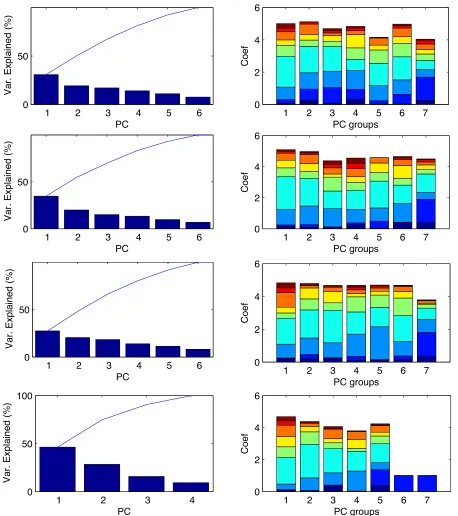
should be combined into one variable or if there are clear relationships to drinking apparent. We assessed the new composite scores’ relationship with each other and with the number of drinks consumed in several time periods and compare to the strength of relationships seen between data from individual questions using inspection, linear interpolation, and principal component analysis. It was previously determined based on existing literature and discussion that time of day is related to the number of drinks a person consumes and thus including time in the study of any other composite scores’ relationships with number of drinks may be important. Additionally, it allows us to see any possible changes in the data - drink relationships as a function of time.
5.1 Initial inspection of the data
Visual interpretation of the data is useful when searching for trends that may not be easily detected or expressed by statistical means and is a logical starting point when investigating a large data set. In our initial search, we detected several trends that should be considered when building our conceptual and mathematical models. Sometimes, relationships between data categories were observed on a short time scale of typically less than two days. Some individuals exhibited similar trends in behavior, indicating that they may be grouped into cohorts at a later stage that may affect the compartments of our conceptual model or how those compartments are related. Finally, different temporal trends in the data became clear at different scales.
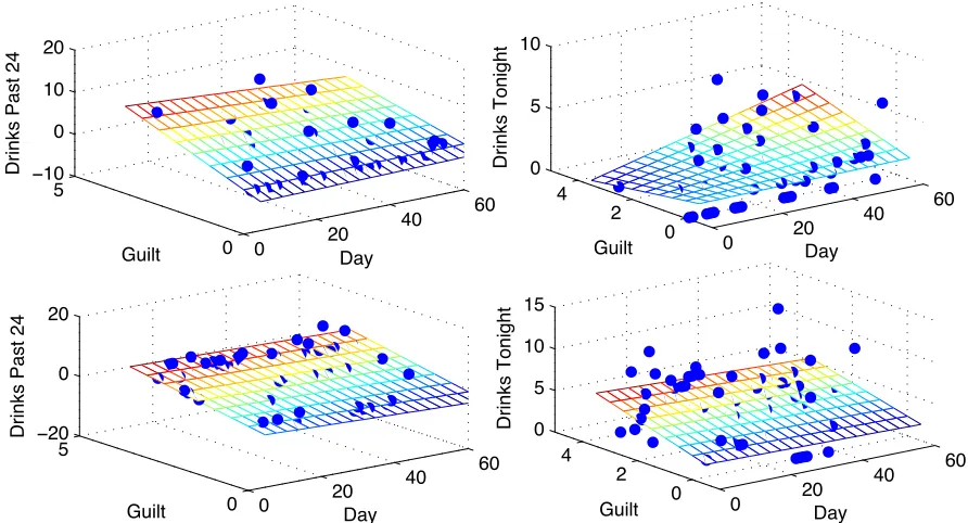
appear stronger or weaker (Figures 6, 7, 8). Figure 6 shows that guilt has a clearer relationship with number of drinks over the past 24 hours than drinks consumed during the evening after the survey for two participants, while Figure 8 indicates that a person’s stress level is related to drinks consumed over the whole day, including the day leading up to and evening following the survey, more strongly than it is related to drinks consumed the night before. The pairing of a category and time period that seems to have the strongest relationship with drinking is located in Table 2.
0 20
40 60
0 5
−10
0 10 20
Day Guilt
Drinks Past 24
0 20
40 60
0 2 4 0 5 10
Day Guilt
Drinks Tonight
0 20
40 60
0 5
−20
0 20
Day Guilt
Drinks Past 24
0 20
40 60
0 2 4 0 5 10 15
Day Guilt
Drinks Tonight
0 20 40 60 0 5 0 5 10 15 Day Desire
Drinks Last Night
0 20 40 60 0 5 0 10 20 Day Desire
Drinks All Day
0 20 40 60 −2 0 2 0 5 10 Day Desire
Drinks Last Night
0 20 40 60 −2 0 2 0 5 10 15 Day Desire
Drinks All Day
Figure 7: Desire versus drinks last night (left) and drinks over all of today (right) for participants 6021 (top) and 6072 (bottom).
0 20 40 60 0 2 4 0 5 10 Day Stress
Drinks Last Night
0 20 40 60 0 2 4 0 10 20 Day Stress
Drinks All Day
0
50 1 2
3 4 0 5 10 Stress Day
Drinks Last Night 0
20 40 60 0 2 4 0 10 20 Stress Day
Drinks All Day
Table 2: Best time period for each observed data category
Data Category Time Period
Events (Stressful and Pleasant) Past 24 hours
Pressure Past 24 hours
Events last night Last night
Events today All of today
Pressure last night Last night
Pressure today Today
Mood Past 24 hours
Stress All of today
Desire All of today
Guilt Past 24 hours
Commitment All of today
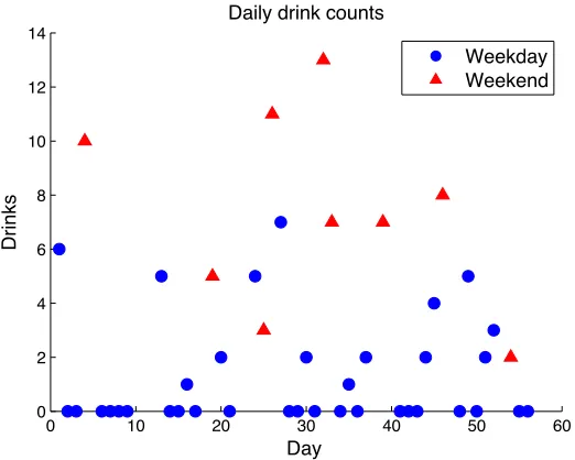
While looking at drinking patterns on this daily or even twice-daily level, we noticed that people show different drinking trends depending on the time of day. Some people tend to be night drinkers and other people appear to be day drinkers. Namely, a participant may exhibit a pattern of being in many more drinking situations or consuming more drinks during one part of the day than the other (Figures 9, 10). In Figure 7, we see that the desire of patient 6021 is related to the drinks 6021 consumed the night before, but the desire of patient 6072 is more closely related to the drinks consumed over the whole day, both before and after the IVR survey. These signs helped us determine that we should first build a number of individual-level models before attempting cohort or population models.
0 10 20 30 40 50 60
0 2 4 6 8 10 12 14
Day
Drinks
Drinks LN Drinks Today
0 10 20 30 40 50 60
0 2 4 6 8 10 12 14
Day
Drinks
Drinks LN Drinks Today
Figure 9: Drinks over time for participants 6021 (left) and 6090 (right).
0 20 40 60 0
0.1 0.2 0.3 0.4 0.5 0.6 0.7 0.8
Day
Pressure
Pressure LN Pressure Today
0 20 40 60
0 0.1 0.2 0.3 0.4 0.5 0.6 0.7
Day
Pressure
Pressure LN Pressure Today
Figure 10: Pressure last night and pressure today over time for participants 6002 (left) and 6090 (right).
drinks consumed on that day or night. It is expected that people behave differently on weekends, which consists of a couple of days. In particular, a person typically does not work on the weekends and thus lacks a particular stress that may induce or suppress the desire to drink; however, that person may spend much more of the day around friends and family, and without the obligation of work, a person may feel more inclined to drink. In our initial explorations of the data, we found that that some people may change their drinking habits over the weekend, but other people do not change (Figure 11). This is yet another indication that the behavior of different individuals would be better reflected using different models.
0 20 40 60 0
5 10 15 20
Day
Drinks all Day
0 20 40 60
0 2 4 6 8 10 12
Day
Drinks all Day
0 20 40 60
2 4 6 8 10 12 14 16
Day
Drinks all Day
Figure 11: Drinks per day over time for participants 6029 (left), 6072 (center) and 6021 (right). Red dots indicate weekend days, and blue dots indicate weekdays.
0 10 20 30 40 50 60
0 2 4 6 8 10 12 14
Day
Drinks
Daily drink counts
Weekday Weekend
0 10 20 30 40 50 60 1
1.5 2 2.5 3 3.5 4 4.5 5 5.5
Day
Drinks
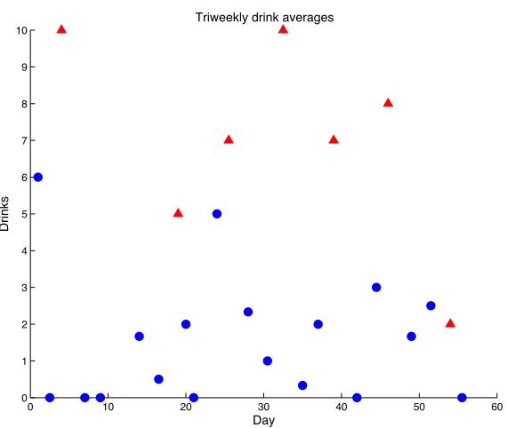
Weekly drink averages, 6029
Figure 13: Average drinks per weekly time period for patient 6029.
0 10 20 30 40 50 60
0 1 2 3 4 5 6 7 8 9 10
Day
Drinks
Triweekly drink averages
5.2 Linear interpolation methods
Scatter plots, multivariate linear regression, and coefficients of determination are the first tools we used to inform us of relationships between data and also between data categories. We examined scatter plots of time versus an observed data category versus drinks and the two dimensional projections in each direction. Multivariate regression methods help to reveal this same dynamic. Regression models are in the form of
f(x, t) =c0+c1t+c2x+c3xt, (1)
which is an affine transformation if the interaction term xtis considered as its own dimension.
First we examined affine relationships between two data columns – either from the original data
set or from the averages across a category – by settingc1 =c3 = 0 and between a data column and
time by setting c2 =c3= 0. Since these simple models did not adequately describe trends seen in
the data, we turned to the full regression model (1). To judge the strengths of these relationships we utilized the coefficient of determination.
The coefficient of determination r2 is used to describe the strength of an affine relationship
between two observed data categories by formulating an affine modelf(x) =ax+bwherea, b∈R
and then measuring the difference between the actual values yi observed at xi and f(xi). These
differences are squared and sum, and this sum is then divided by the sum of the squared differences
between the mean ¯y and each yi, thus normalizing the value of variance explained by f(x) by the
total variance seen in the data set of allyi. The coefficient of determination is calculated via
r2 = 1−
n
i=1(yi−f(xi))2
n
i=1(¯y−yi)2
wherenis the number of data points, xi is the explanatory variable value, yi is the corresponding
response variable value, and f(xi) is the predicted response variable value given xi and the affine
transformationf calculated in MATLAB. The determination of explanatory variables and response
variable in this procedure is arbitrary and thus r2 provides no information on the direction of the
relationship.
Since we expected that different participants in Project MOTION possess different
characteris-tics, we focused on finding coefficients of determination for individual data sets and calculater2for
the categories. We sought strongly (r2 >0.50) affine relationships and weaker (0.20 < r2 <0.50)
affine relationships. Note we could not account for any relationships that may vary with time or non-affine relationships such as polynomial of order two or greater or exponential relationships.
5.2.1 Interpolation of original IVR data
We focused our search for linear relationships on the IVR data from the previously mentioned 11 participants who decreased their drinking over the course of Project MOTION. These 12 partici-pants had relatively complete data: they each started the survey at least 35 out of 56 times and failed to complete the survey no more than twice. The data of these participants show different trends and the correlation matrices for one dimensional linear relationships for each individual differ greatly, indicating that each of these individuals operate by different underlying mechanics.
The average r2 across individuals, however, indicated that only 3 relationships are strongly affine