Model Development for Shape Memory Polymers

SISKIND, RYAN D. Model Development for Shape Memory Polymers. (Under the direction of Professor Ralph C. Smith).

Shape memory polymers (SMPs) have garnered a considerable amount of atten-tion in recent years due to their flexible, lightweight, and biodegradable nature. At high temperatures, SMPs share attributes with compliant elastomers and exhibit long-range re-versibility. In contrast, at low temperatures they become very rigid and are susceptible to plastic, although recoverable, deformations. Their ability to withstand large, nonlin-ear deformations coupled with their ability to completely recover their original shape is of particular interest for biomedical, aerospace, and automotive applications. Whereas the scope of existing models involving isothermal nonlinear deformations at both high and low temperatures is broad, there is a noted lack of models which specifically deal with the transition process. This process cannot be overlooked as it is the driving factor for all thermomechanical shape memory effects in shape memory polymers.

by

Ryan David Siskind

A dissertation submitted to the Graduate Faculty of North Carolina State University

in partial fullfillment of the requirements for the Degree of

Doctor of Philosophy

Applied Mathematics

Raleigh, North Carolina

2008

APPROVED BY:

Dr. Stefan Seelecke Dr. Hien Tran

DEDICATION

BIOGRAPHY

Ryan David Siskind is the youngest of Harry and Claudia Siskind’s three children. He was born on November 22, 1980 and was raised in Willoughby, Ohio. While attending Willoughby South High School, he discovered his penchant for music and the sciences. After graduating high school in 1999, he attended Youngstown State University with an undeclared major and the desire to explore his musical and scientific talents further. After only one term, it was clear that mathematics came naturally and he declared it his major in early spring. He spent the remaining three-and-a-half years taking as many math classes as possible, exhausting the undergraduate catalog before his senior year.

Ryan earned his bachelors in Mathematics in 2003 and, because he didn’t spend enough time thinking about what he was going to do with a degree in mathematics, he decided to pursue his PhD and was accepted at North Carolina State University. It was there that he grew a love for the practical applications of Applied Mathematics and began researching shape memory polymers in the summer of 2006 under the direction of Dr. Ralph Smith.

ACKNOWLEDGMENTS

I cannot begin without expressing the amount of gratitude I have for my adviser, Dr. Ralph C. Smith. I thought he was crazy when he promised I could earn a diploma within two years of starting research under him, but he kept that promise. He had the unenviable job of keeping me on task, encouraging me when I hit the doldrums, and inventing stories to tell my girlfriend about why I would be out of town for no good reason (even though that reason was to ask her parents for permission to marry her). For this and much more, I will be eternally grateful.

I also extend my deepest gratitude to Dr. Mansoor Haider, Dr. Stefan Seelecke, Dr. Kazufumi Ito, and Dr. Hien Tran, all who served in some capacity on my committee.

The faculty and (most importantly) the staff of the Mathematics department are truly top-notch. Whether I was a student, a subordinate, a colleague, or an absolute annoyance, their wisdom and support helped me through hard times; both personal and secretarial.

To my family: Whether you are a Siskind, Pasiechnik, Dingledein, Braund, Hart, Morgan, McDerment, Sweetapple, Pim, Cirnski (and more), you have always been the most important part of my life and will continue to be for the rest of it. Thank you not only for your love and support, but for your time and patience.

To my family members whom I dearly miss, Grampa Honey, Auntie Kris and Grampa Siskind: I know you are watching and guiding me from the cloud tops. . . I only wish I could see your smiles and feel your hugs one last time.

To all of my friends. . . there are too many to name, so I will just say one giant thank you. I couldn’t have survived the agony of school without your compassion, humor, or livers.

stop loving me. And I will never stop loving him.

TABLE OF CONTENTS

LIST OF TABLES . . . viii

LIST OF FIGURES . . . ix

1 Introduction . . . 1

1.1 SMA shape recovery process . . . 6

1.2 SMP shape recovery process . . . 7

1.3 Comparison of SMPs with SMAs . . . 9

1.4 Modeling Techniques . . . 10

2 A Homogenized Model for Deformations in SMPs . . . 11

2.1 Introduction . . . 11

2.2 Thermal Strain . . . 15

2.3 Polymer Network . . . 16

2.4 Cooling a Polymer Network . . . 18

2.4.1 Homogenized Cooling Thermal Strain . . . 18

2.4.2 Homogenized Cooling Mechanical Strain . . . 19

2.4.3 Homogenized Cooling Stored Strain . . . 20

2.4.4 Homogenized Model for Cooling a Polymer Network . . . 24

2.4.5 Cooling with Constant Strain . . . 24

2.5 Heating a Polymer Network . . . 26

2.5.1 Homogenized Heating Thermal Strain . . . 26

2.5.2 Homogenized Heating Mechanical Strain . . . 27

2.5.3 Homogenized Heating Stored Strain . . . 27

2.5.4 Recovered Strain . . . 29

2.5.5 Homogenized Model for Heating a Polymer Network . . . 32

2.6 Glass Transition Phenomenon . . . 33

2.6.1 Polydispersity . . . 33

2.6.2 Tan δ. . . 35

2.6.3 Modeling tan δ. . . 37

2.7 Thermodynamic Considerations . . . 43

2.8 Model Properties . . . 46

2.8.1 Unconstrained Thermocycle . . . 47

2.8.2 Cooling with Static Applied Force . . . 47

2.8.3 Unconstrained Heating . . . 48

2.8.4 Predicted Thermomechanical Cycle . . . 48

2.9 Thermomechanical Experimental Validation . . . 50

2.9.1 Fully Constrained Cooling . . . 51

2.9.2 Recovery Heating. . . 54

3 Shape Memory Polymers in a Rod System . . . 59

3.1 Introduction . . . 59

3.2 Rod Model Setup . . . 60

3.3 Homogenized SMP Model . . . 62

3.4 Weak Formulation using Constitutive SMP Model . . . 64

3.5 Numerical Methods . . . 65

3.5.1 Gaussian Quadratures . . . 66

3.5.2 Trapezoid methods . . . 66

3.5.3 Rosenbrock-Type Methods . . . 69

3.6 Model Implementation . . . 70

3.6.1 Stability concerns . . . 71

3.6.2 Implementation using Rosenbrock Method . . . 73

3.7 Experimental Procedure . . . 76

3.7.1 Isothermal tension and compression . . . 76

3.7.2 Unconstrained cooling and heating . . . 77

3.7.3 Glass transition . . . 77

3.7.4 Constrained heating. . . 79

3.8 Homogenized rod model prediction . . . 80

3.8.1 Model Validation . . . 80

3.9 Model Properties . . . 81

3.10 Conclusion . . . 82

4 Models for Large Strain in Polymers . . . 84

4.1 Models for Large Strain in Active Polymers . . . 85

4.1.1 Mathematics of a Single Chain . . . 85

4.1.2 Linearization for Small Strains . . . 89

4.2 Network Models . . . 90

4.2.1 3-Chain Model . . . 91

4.2.2 8-Chain Model . . . 91

4.2.3 Model Validation using Tension Tests . . . 92

4.2.4 Full Network Model . . . 96

4.3 Models for Large Strain in Frozen Polymers . . . 99

4.3.1 Intermolecular Resistance to Flow . . . 100

4.3.2 Moleculuar Alignment . . . 100

4.3.3 Finite Strain Kinematics . . . 101

4.3.4 Phenomenological exponential model . . . 102

5 Conclusion . . . 105

LIST OF TABLES

Table 2.1 Initial and optimized values for a single distribution along with respective errors . . . 40 Table 2.2 Initial and optimized values for a Galerkin approximation along with respective

errors . . . 41

LIST OF FIGURES

Figure 1.1 Photoresponsive crosslinking agent azo-dye . . . 2

Figure 1.2 SMP foam in a compact form . . . 2

Figure 1.3 SMP temperature-dependent modulus . . . 3

Figure 1.4 SMP stent . . . 4

Figure 1.5 SMP suture . . . 5

Figure 1.6 Cornerstone Research Group SMP wing . . . 5

Figure 1.7 Possible SMP space applications . . . 6

Figure 1.8 SMA cellular configurations . . . 7

Figure 1.9 Thermomechanical cycle of a smart materials . . . 7

Figure 1.10 Coexisting frozen and active portions of a polymer . . . 9

Figure 2.1 Typical thermomechanical cycle of a shape memory polymer. . . 13

Figure 2.2 Thermal strain via curve fitting . . . 15

Figure 2.3 Thermal strain of a single SMP element . . . 16

Figure 2.4 A polymer network composed ofN homogenous elements. . . 17

Figure 2.5 Cooling a single SMP element . . . 21

Figure 2.6 Thermal recovery strain of a single SMP element . . . 30

Figure 2.7 Mechanical recovery strain of a single SMP element . . . 31

Figure 2.8 Total recovery strain of a single SMP element . . . 32

Figure 2.9 Polydispersity relation for polymers . . . 34

Figure 2.10 Tanδ data . . . 36

Figure 2.12 Single distribution initial estimate of tan δ . . . 38

Figure 2.13 Adjusted tanδ data . . . 39

Figure 2.14 Approximations of adjusted tanδ data . . . 41

Figure 2.15 Decomposed Galerkin approximation of adjusted tanδ data . . . 42

Figure 2.16 Frozen fraction during cooling and heating . . . 43

Figure 2.17 Tanδ approximations with corresponding frozen fractions . . . 44

Figure 2.18 Homogenized model’s prediction of thermal strain . . . 48

Figure 2.19 Homogenized model’s prediction of constrained cooling . . . 49

Figure 2.20 Homogenized model’s prediction of unconstrained heating . . . 49

Figure 2.21 Typical observed thermomechanical cycle . . . 50

Figure 2.22 Liu’s thermomechanical experiments . . . 52

Figure 2.23 Isothermal stress-strain relation . . . 53

Figure 2.24 Unconstrained cooling experiment . . . 53

Figure 2.25 Model’s prediction of the constrained cooling . . . 54

Figure 2.26 Comparison of Liu’s model with the homogenized model . . . 55

Figure 2.27 Model’s prediction of unconstrained and constrained heating . . . 56

Figure 2.28 Constrained heating with dynamicαf . . . 56

Figure 2.29 Liu model prediction of unconstrained and constrained heating . . . 57

Figure 3.1 Space boom . . . 60

Figure 3.2 Rod model structure . . . 60

Figure 3.3 Region of stability for explicit trapezoid method . . . 69

Figure 3.4 Comparing implicit and explicit trapezoid method . . . 73

Figure 3.5 Isothermal stress-strain experiments . . . 77

Figure 3.7 Tanδ experiments . . . 78

Figure 3.8 Partially constrained recovery . . . 79

Figure 3.9 Model prediction of partially constrained recovery . . . 80

Figure 3.10 Theoretical cooling strain . . . 82

Figure 3.11 Theoretical heating strain . . . 83

Figure 4.1 Single chain based on the assumptions of Kuhn and Gr¨un . . . 86

Figure 4.2 Chain orientation for the (a) 3-chain and (b) 8-chain models. . . 92

Figure 4.3 Uniaxial and Biaxial data collected by Treloar . . . 93

Figure 4.4 Data comparison with the 3-Chain model . . . 95

Figure 4.5 Uniaxial and Biaxial model comparison for 3-Chain model . . . 95

Figure 4.6 Data comparison with the 8-Chain model . . . 96

Figure 4.7 Uniaxial and Biaxial model comparison for 8-Chain model . . . 97

Figure 4.8 Plastic deformation of an SMP under compression . . . 99

Chapter 1

Introduction

Shape memory polymers (SMPs) are a class of smart materials that have recently garnered a large amount of interest for their possible use in mechanical systems due to their lightweight, flexible, cost-effective, and highly deformable nature. They are non-metallic in nature and each SMP can be classified by the stimulus which creates a shape memory response.

Photoresponsive and chemoresponsive polymers are materials which change shape due to exposure to light or chemicals respectively. The most basic photoresponsive poly-mer contains the crosslinking agent azo-dye (N=N group) which gives each crosslink a cis-trans isomerism property [26]. The trans form of the isomer has a molecular length of approximately 9˚A (Figure 1.1(a)) and the cis form of the isomer has a molecular length of approximately 5.5˚A (Figure 1.1(b)) . When left unexposed to light, the cis and trans forms coexist. When irradiated with ultraviolet light, the cis form becomes dominant causing the polymer to contract. Upon irradiation with visible light, the trans form is dominant causing the polymer to expand. Figure 1.1 illustrates how utilizing the cis-trans isomerism of the azo-dye crosslinking agent can create displacement in a polymer.

Chemoresponsive polymers contain a reactive pendant group which cause the poly-mer to dissociate into ions when the pH of the surrounding medium is changed [26]. When crosslinked, these polymer networks comprise a gel or a film which, when submerged in water, changes shape when an acid or alkali is introduced into the water due to the ionic forces created between the polymer chains.

N N = 9.0A

o

(a)

N

N

=

5.5A

o

(b)

Figure 1.1: The crosslinking agent azo-dye as (a) the trans isomer with a molecular length of 9˚A and, (b) the cis isomer with a molecular length of 5.5˚A.

foams and gels comprise a group of thermally-induced shape memory polymers which dras-tically change volume. Some gels can swell or shrink by up to a factor of three [45]. When heated, polymer foams can be compacted into very small volumes relative to their original size and subsequently cooled to retain the compact shape. Upon reheating, the foam will return to its original volume and shape. Figure 1.2 illustrates the ability of a polymer foam developed by Cornerstone Research Group to sustain a considerable decrease in volume. The ability of foams to retain their compact shape illustrates the phenomenon known as glass transition in polymers.

One of the most prominent features shape memory polymers exhibit is a dramatic change in modulus as a result of temperature change. At high temperatures, polymers exist

in a very compliant, malleable state. Conversely at low temperatures, polymers exist in a rigid state. The modulus of the polymer can increase between 100 and 1000 times when cooled and it is due to this change in modulus that deformations, much like the polymer foam’s compacted state, can be locked into place when the polymer is cooled. Figure 1.3 shows the modulus of a typical shape memory polymer over a wide temperature range. There are three distinct regions: a high modulus plateau below the glass transition, the glass transition region, and a low modulus plateau above the glass transition. As a point of reference, it is common to describe the glass transition region by a point termed the glass transition temperatureTg which exists somewhere in the transition region (the definition of which varies widely in the literature). Temperatures termed “high” and “low” are always material-dependent based on the glass transition region. A temperature of 273◦_{K (0}◦_{C) is}

considered a high temperature for polyethylene whose glass transition temperature is 168◦_K

but is considered low for polycarbonate whose glass transition temperature is 418◦_K.

Two types of thermomechanical polymers are of particular interest due to their solid structures; thermoplastic and thermoset polymers. Thermoplastic polymers are solid polymers that possess drastically different properties depending on the operating tempera-ture, but also possess the ability to melt at high temperatures. While in the melted state, the polymer exhibits a cohesive nature due to crosslinking and physical entanglements of polymer chains, is easily remolded into different shapes, and has the ability to be welded

260 280 300 320 340 360

100 101 102 103 104

Temperature (K)

Modulus (MPa)

High Modulus

Glass Transition

Low Modulus

Tg

with other thermoplastic polymers. Some examples of thermoplastic polymers are poly-ethylene, polypropylene, poly(methyl methacrylate) (PMMA, more commonly known as Plexiglas), and polycarbonates.

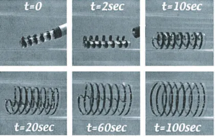
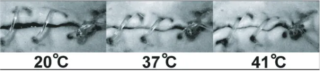
Thermoset polymers, unlike thermoplastics, cannot melt to be remolded or welded with other polymers; however, thermoset polymers tend to be much stronger than thermo-plastic polymers. It is this classification of polymer which constitutes the bulk of research conducted for this dissertation. Biomedical applications involving thermoset SMPs already exist due to their biodegradability and their ability to be temporarily stored in a compact shape, implanted with minimally invasive surgery, and subsequently reheated in vivo in a controlled process to return to its original shape. Figure 1.4 illustrates how a stent made from a shape memory polymer [49] can be deployed in a compact shape and, through a slow and controlled release, recovers to its original shape. Shape memory polymers can also be implemented as sutures to aid in surgical procedures where working room is at a premium. Figure 1.5 shows how a shape memory polymer wire can be implemented as pre-stretched sutures [30]. After closing a wound, the suture can be slowly heated to contract to its original length and as a result, the wound is closed tighter.

Thermoset shape memory polymers are also being investigated for larger structural purposes. Aerospace industries are investigating the use of shape memory polymers as mold-able skin for adaptmold-able wings that can dynamically change their shape in order to optimize the aerodynamic properties of the wing during flight. Military applications involve the compact deployment of large structures such as bridges and drone planes (www.crgrp.com). Figure 1.6 shows how a wing can be compactly stored and subsequently heated to return

to its original, aerodynamic state. The concept for this wing was developed by Cornerstone Research Group using their high-performance suite of shape memory polymers including the polymer Veriflex, dynamic composite Veritex, and syntactic foam Verilyte.

The weightlessness of space can easily support enormous manmade structures, however the fabrication of such structures is still a terrestrial task. The ability to transport these structures is problematic due to the weight and size. Using shape memory polymers, the feasibility to construct large, lightweight structures that possess the ability to be com-pacted into small volumes is currently being explored. Deployable systems such as satellite dishes, solar sails, or solar arrays can be folded or rolled into compact sizes for shipment and, once in space, can recover their full size and shape. Figure 1.7(a) illustrates the deployment of a shape memory polymer membrane developed by Cornerstone Research Group. Booms and antennas are also necessary structures for space applications, however their size limits the usefulness of their application. Figure 1.7(b) shows a standard triangular layout for an antenna which can integrate shape memory polymers into its longerons, battens and cross

Figure 1.5: A prestretched suture can be used to loosely close a wound, and when subse-quently heated it will return to its original length, tightly closing the wound [30].

(a) SMP membrane

Longeron

Batten

Cross Member

(b) Antenna

Figure 1.7: Possible space applications for shape memory polymers including (a) a mem-brane for satellites or solar sails (Cornerstone Research Group), and (b) an antenna or boom.

members. Doing so could allow folding and rolling to minimize the volume necessary to transport such a structure.

Before applications of shape memory polymers becomes commonplace, it is neces-sary to characterize the thermomechanical properties in order to accurately predict how a polymer will respond to stimulus. It is impossible to ignore the correlation between shape memory alloys (SMAs) and shape memory polymers, and with the wealth of information on their thermomechanical behavior, we will begin by summarizing the shape recovery process of SMAs.

1.1

SMA shape recovery process

Shape memory alloys are smart materials that are metallic in nature and whose shape recovery processes are enthalpy driven. The behavior of shape memory alloys is dictated by transformations from a high symmetry austenite phase to lower symmetry martensite phases. Figure 1.8 illustrates these cellular configurations.

(a) (b) (c)

Figure 1.8: (a) Austenite, (b) twinned martensite and (c) detwinned martensite cellular configurations of a shape memory alloy.

s

e

T

T

1

2

3

4

(a)

s e

T

g

1

2

3

4

T

(b)

Figure 1.9: Comparison of thermomechanical cycles for (a) shape memory alloys [39] and (b) shape memory polymers [31].

Once the alloy is belowTtr, it is deformed with an applied stress (or strain). This applied deformation causes a strain (or stress) on the alloy which grows linearly until a critical stress is reached at which point the twinned martensite transitions to the detwinned martensite cell configuration. After the transition to the detwinned state, the applied defor-mation is released but a residual strain remains because of the detwinned martensite cellular configuration. In the final step of the shape recovery process, the alloy is heated above Ttr at which point the martensite configuration returns to the stable austenite configuration.

1.2

SMP shape recovery process

chains, cross-linking, crystallization and the formation of domain structures. These inherent physical interactions give each SMP unique properties but, due to their polymeric nature, the overall shape recovery process is similar. When a deformation is applied to a polymer, the molecular chains move to accommodate the new configuration. Because the deformation creates an ordered motion of molecules, the number of possible configurations a single chain can attain decreases. The result is a decrease in configurational entropy and the force in the chain is not cause by a change in energy, but a change in entropy. Because of this distinction, shape memory polymers are considered to be entropy driven.

The typical shape recovery process for small deformations, shown in Figure 1.9(b), begins at a temperature above the glass transition temperature, Tg. At this temperature, the polymer is in a rubbery elastic (active) state. The polymer is then deformed with an applied stress (or strain) which creates a strain (or stress) in the polymer.

Once the polymer is deformed, it is cooled belowTgat which point the active poly-mer becomes inelastic (frozen or glassy). The applied deformation is removed; however, the polymer does not return to its original configuration because a portion of the deformation becomes “locked” in place below Tg. The resulting deformation creates a residual strain which remains present until the shape recovery process is completed when the polymer is heated above Tg.

It is important to note that polymers at low deformation levels (compared to what they are capable of sustaining) exhibit a fully recoverable linear elastic behavior. If an undeformed polymer is cooled belowTg and then stressed, it will return to its previous undeformed state upon removal of the stress. The yield in SMAs as a result of cellular re-configuration (illustrated in part 2 of Figure 1.9(a)) does not occur in SMPs until molecular reconfiguration is achieved. Typically this does not happen until a strain of 20% or more is applied.

While the shape recovery process of shape memory alloys is a result of different cellular configurations in which they can exist, the recovery in SMP is governed by the transition from an active state to a frozen state (and back again). It is widely accepted that both the active and frozen states can coexist during the glass transition process resulting in a temperature range, rather than a point, where a polymer’s properties transition. This is illustrated in Figure 1.3 where the modulus of the polymer transitions for almost 30◦ _before

Figure 1.10: Coexisting frozen and active portions of a polymer [31].

1.3

Comparison of SMPs with SMAs

Shape memory alloys are widely used and known to have large recovery pressures (as much as 500 MPa). When thermomechanically driven, they are able to conduct heat very well. They are also able to dissipate energy effectively when going through the shape recovery process. However, SMAs are only able to recover from deformations up to 10%, above which plastic deformation with unrecoverable shape change can occur. Also, they are subject to internal heating and metal fatigue, both of which degrade the reliability of SMAs.

1.4

Modeling Techniques

Currently, the thermomechanical modeling of shape memory polymers can be clas-sified into four categories: isothermal nonlinear plastic deformations for large strains at temperatures below Tg, isothermal nonlinear elastic deformations for large strains at tem-peratures aboveTg, the strain storage process of linear deformations which bridge the glass transition gap, and the strain storage process of nonlinear deformations which bridge the glass transition gap.

Due to their ability to fully recover from large deformations, a considerable amount of research has been conducted on large strain, isothermal deformations in shape memory polymers. Applications which involve folding or rolling polymers requires strains above 20%, well within the nonlinear range of deformations; however, the amount of research involving the strain storage and recovery characteristics is notably lacking. The glass transition process is not well understood and, as a result, quantifying how a deformation is locked into place is difficult. In the following chapters, we explore these and other open questions regarding the thermomechanical shape recovery process of shape memory polymers.

Chapter 2

A Homogenized Model for

Temperature-induced

Deformations in Shape Memory

Polymers

2.1

Introduction

Whereas the research involving shape memory polymers (SMPs) is less mature than that of shape memory alloys (SMAs), the proposed uses for these materials demon-strate significant potential. Polymer medical sutures that are stretched and locked in an elongated state utilize a temperature-controlled release to return to their original length [30]. If this recovery process is implemented after the suture is used to close a skin lacera-tion, a tighter stitch is possible. Polymer sutures can also be used where the parent shape is a loose knot [30]. Locking the suture in a straightened state prior to use allows for wound closure in tight areas where tying a finishing knot is difficult or impossible. Once the suture is made, again through a temperature-controlled release, the free end wraps around itself into a loose knot.

each wing needs to be a very pliable yet rigid material and SMPs exhibit both characteristics when transformed through different temperature regimes.

Space systems necessarily need to utilize smart materials due to their immense size once fully operational. The lightweight, flexible, cost effective, and highly deformable nature of SMPs make them a leading candidate in the development of space systems[45]. For example, deployable antenna booms with rigid battens can be constructed with SMP joints. These joints can be bent prior to deployment in order to minimize the fully assembled volume necessary for transport. Once in space, the polymer joints are returned to their parent shape, allowing the antenna to reach its fully deployed shape.

The scope of models that focus directly on temperature-induced deformations is much smaller than their isothermal counterparts. Several existing phenomenological models define the total strain ε as the sum of the thermal, mechanical and stored strains, respec-tively denoted byεT, εm and εs, so that

ε=εT +εm+εs. (2.1)

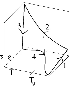
It is the constitutive definitions of these strains that are addressed. A typical thermome-chanical cycle for a shape memory polymer is shown in Figure 2.1. Beginning at a high temperature where the polymer exhibits rubbery elastic properties, the polymer is deformed (1). Once a desired deformation is achieved, it is held constant while the temperature is decreased. As the temperature decreases, the modulus of the polymer markedly increases (between two and three orders of magnitude) and the polymer becomes rigid. Once the entire polymer has reached a low temperature, the deformation is released and a fixed de-formation is observed as a result of the increased modulus (3). The polymer is then heated to the original high temperature, releasing the fixed deformation and allowing the polymer to return to its original shape (4).

s e

T

g

1

2

3

4

T

Figure 2.1: Typical thermomechanical cycle of a shape memory polymer.

Therefore, the model defined by Liu is given as

εT(T) = (1−φf(T))εaT(T) +φf(T)εfT(T), εm(T, σ) = (1−φf(T))εam(T, σ) +φf(T)εfm(T, σ), dεs

dT(T, σ) =

Y(T) Ya(T)

(ε₋εs(T, σ)−εT(T)) dφf

dT (T)(T), εs(T0) = 0,

whereT is the absolute temperature,εis the constant strain during cooling, andY(T) and Ya(T) are the temperature-dependent moduli of the bulk polymer and active portion of the bulk polymer respectively. The internal state variableφf(T) defines the frozen fraction and is essential in the strain storage process.

model is given as

εT(T(t)) = [1−φf(T(t))]εaT(T(t)) +φf(T(t))εf_T(T(t)) +

Z T(t)

T0

(εa_T(θ)₋ε_Tf(θ))φ0_f(θ) dθ,

εm(T(t)) =

1₋φf(T(t)) Ya(T(t)) −

φf(T(t)) Yf(T(t))

σ(t),

εs(T(t)) =

Z t

0

1 Ya(T(τ)) −

1 Yf(T(τ))

σ(τ)dφf

dT (T(τ))Te

0_(τ)dτ,

where T is the absolute temperature, εa

T and εfT are the respective thermal strains of the active and frozen volumes, Ya and Yf are the respective moduli of the active and frozen volumes,φf is the frozen volume fraction, andTe0 is the change in the temperature history with respect to time (see [10] for details).

The Chen-Lagoudas model is similar to the Liu model and differences can be attributed to Liu’s simplification of part of the freezing processes. Whereas these models predict the overall thermomechanics of a shape memory polymer’s shape recovery process, both models rely on curve fitting to define several of their key elements. Because the glass transition does not necessarily overlap during cooling and heating [34], the process of strain storage and release may exhibit some hysteresis. Underlying physical properties, including strain relaxation and shifts in the glass transition due to pressure, are nominalized when curve fitting is applied universally. The goal of defining a model that relies on data strictly for parameter estimation and model calibration is the basis of this chapter.

2.2

Thermal Strain

The total thermal strainεT is constitutively defined in [32] as

εT(T) = (1−φf(T))εaT(T) +φf(T)εf_T(T) =

Z T

T0

[(1₋φf(θ))αa(θ) +φf(θ)αf(θ)]dθ.

An unconstrained cooling experiment was conducted where it was assumed the sole internal straining mechanism was thermal strain. This led to a simplified definition of thermal strain

εT =

Z T

T0

α(θ) dθ,

where the thermal expansion was found via curve fitting to have the functional relation α(T) =₋3.16_×10−4+ 1.42_×10−6T

as shown in Figure 2.2. This relation, however, does not take into account the storage process which occurs upon cooling through the glass transition.

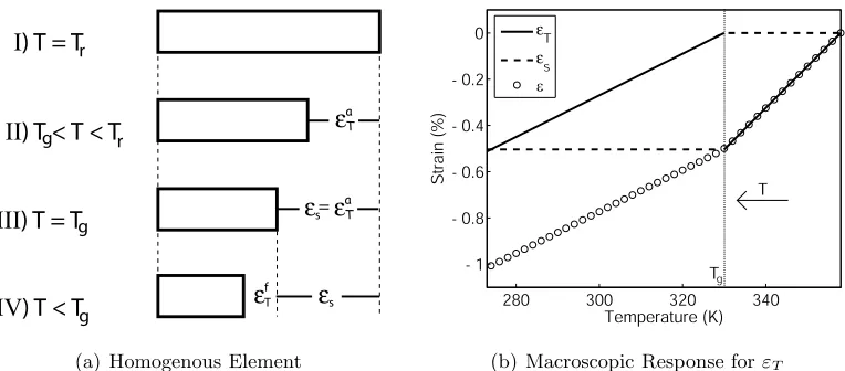
To illustrate, consider a single polymer element with total strain as given in (2.1) which is being cooled with no externally applied forces (thus εm = εam = εfm = 0) as shown in Figure 2.3(a). The single polymer element is defined to have a glass transition point at Tg so that φf = 1 for T < Tg and φf = 0 for T > Tg. The element begins in a reference configuration (I) at the reference temperature Tr. As thermal strain is created by

280 300 320 340

-10 -8 -6 -4 -2

x 10 -3

Temperature (K)

Strain

e T Data Curve Fit

e

T= 7.1140x10 T - 3.1550x10 T + 0.0217

-7 2 -4

e_s

g I_{) T = T}

IV_{) T < T} III_{) T = T} r

g

g

eaT

eaT

e_s =

ef_T II_{) T < T < T}

r

(a) Homogenous Element

280 300 320 340

- 1 - 0.8 - 0.6 - 0.4 - 0.2 0

Temperature (K)

Strain (%)

e T e

s ε

T

T_g

(b) Macroscopic Response forεT

Figure 2.3: A single homogenous polymer element during a cooling process showing the deformation due to thermal strain given (a) at discrete values of T and (b) for continuous values ofT.

the decreasing temperature, the polymer contracts (II) and the strain isε=εa_T.At T =Tg (III) the evolution of εa_T halts since this is the lowest temperature for which the polymer is active. At a temperature T = Tg−∆T, (2.1) simplifies to ε = εfT +εs; however, the thermal strainεa

T created while in the active phase is not lost. It is instantaneously frozen as stored strain εs at the glass transition point and the thermal strain, defined as εT =εf_T when T < Tg, is again zero atT =Tg−∆T. While the temperature continues to decrease (IV), the stored strain remains constant as the frozen thermal strain develops.

Figure 2.3(b) shows the continuous temperature-induced response for the single homogenous polymer element during a cooling cycle. As previously argued, the thermal strain develops in both the active and frozen states; however the thermal strain instanta-neously returns to zero at the glass transition point. The thermal strain that is ‘lost’ is locked into place in the stored strain allowing a continuous deformation. If each polymer network is considered to be the sum of polymer elements, each with unique properties, the entire network deformation can be considered the average of the elemental deformation.

2.3

Polymer Network

1 2 3 4 . . . N

Figure 2.4: A polymer network composed of N homogenous elements.

glass transition pointTgi with the elemental frozen fraction defined as

φfi(T) =   

0 when T _≥Tgi,

1 when T < Tgi.

The weighted average of these φfi defines the total frozen fraction of the polymer network

so that

φf = N

X

i=1

φfi

`i

`. (2.2)

The strain value of each elementεi is unique in its description since it pertains to the deformation of the specific element. These strain values are defined as

ε= ∆` ` , ε2=

∆`1

`1

, . . . , εN = ∆`N

`N .

To consider each element’s strain contribution to the overall network (i.e., ∆`i/`), we note that the total strain can be expressed as

ε= N

X

i=1

εi `i

`. (2.3)

Since εi denotes the local strain, then εi

`i ` =

∆`i `i

`i ` =

∆`i `

designates how the locally generated strain affects the entire network. This interpretation of strain can be extended to any type of strain generated during a thermomechanical cycle of a shape memory polymer.

Since it is assumed that all active thermal strain is completely stored at the glass transition point, it is not possible to have zero stored strain at a reference temperature below the glass transition point. Also, the frozen and active thermal strains are always considered to be continuous while the total thermal strain is not necessarily continuous.

2.4

Cooling a Polymer Network

To indicate the cooling portion of a thermomechanical cycle, all strain values, glass transition temperatures, and frozen fractions occurring during cooling will be denoted with a ‘-’ in the exponent.

2.4.1 Homogenized Cooling Thermal Strain

Consider the thermal strains generated during a cooling cycle along with the pre-viously defined convention that thermal strain is stored at the glass transition point. The active and frozen thermal strains of the entire network, as previously defined in (2.3), are given respectively as

εa_T− = N

X

i=1

εa_T−

i

`i `,

εf_T− = N

X

i=1

εf_T−

i

`i `.

(2.4)

Assuming a heterogeneous polymer, it can be assumed that the thermal expansion coefficientsαf(θ) andαa(θ) are equivalent throughout the network and thus each element’s thermal strain can be defined as

ε−_T

i = Z T

T−

gi

α(θ)dθ.

To unify the notation for each element in the network, and considering the fact that the network will be uniformly thermally activated, the active and stored thermal strains can be respectively defined as

εa_T−

i (T) = Z T

T−

gi

αa(θ) dθ=

Z T

T0

αa(θ)(1₋φ−_f

i(θ))dθ,

εf_T−

i (T) = Z T

T−

gi

αf(θ)dθ=

Z T

T0

Considering only the active thermal strains (however, the similar treatment can be applied to the frozen thermal strains), (2.4) can be rewritten as

εa_T− = N

X

i=1 Z T

T0

αa(θ)(1−φ−fi(θ))dθ

`i `

=

Z T

T0

αa(θ)

" _N X

i=1

(1₋φ−

fi(θ))

`i `

#

dθ.

(2.5)

Examination of the bracketed term in (2.5) reveals that it represents the active volume fraction of the entire network and can be rewritten as such. Therefore, (2.5) simplifies to

εa_T−(T) =

Z T

T0

αa(θ)(1−φ−_f(θ))dθ. (2.6)

Equation (2.6), along with the frozen thermal strain treated in the same manner, combine via (2.1) to define the total thermal strain of the polymer network as

ε_T−(T) = (1₋φ−_f(T))ε_Ta−+φ−_f(T)εf_T−

= (1₋φ−_f(T))

Z T

T0

αa(θ)(1−φ−f(θ))dθ+φ−f(T)

Z T

T0

αf(θ)φ−f(θ) dθ.

2.4.2 Homogenized Cooling Mechanical Strain Mechanical strain, as defined in [32] and [11], is

ε−_m(T, σ) = (1₋φf(T))εam(T, σ) +φf(T)εfm(T, σ).

It is here that the overall stress-strain relationship is defined. In a general sense, it can be stated that σ = F(T, εm) where F is the standard linear or nonlinear and (possibly) non-invertible stress relation determined by the operating temperature T and the applied mechanical stressεm.Since the basis of this chapter relies on a polymer network reacting in a linear-elastic manner due to relatively small values of strain, the mechanical strain acting on each polymer element can be defined via Hooke’s Law as

εa_m−_i(T, σ) = σ Ya(T) εf_m−_i(T, σ) = σ

where Ya and Yf are the active and frozen moduli of the polymer respectively. Applying (2.3), the mechanical strains are given by

εa_m−(T, σ) = N

X

i=1

σ Ya(T)

`i ` =

σ Ya(T)

εf_m−(T, σ) = N

X

i=1

σ Yf(T)

`i ` =

σ Yf(T)

,

and the total mechanical strain during cooling is ε−_m(T, σ) = 1−φ

−

f(T) Ya(T)

+φf(T)− Yf(T)

!

σ.

2.4.3 Homogenized Cooling Stored Strain

Consider the cooling portion of a thermomechanical cycle on a single element as depicted in Figure 2.5. Beginning with the element in its reference configuration at reference temperatureTr (I), a force is applied (II). The only strain present is the mechanical strain caused by the applied force, εa

m(T, σ). As the element cools towards its glass transition temperature (III), an active thermal strain develops and the strain is

ε(T, σ) =εa_m(T, σ) +εa_T(T). At T =Tg, (IV), the polymer has a total strain of

ε(Tg, σ) =εam(Tg, σ) +εaT(Tg);

however, this amount of strain is not the total strain that is stored during cooling. To properly identify the stored strain, the applied load σ must be removed. This causes the element to “spring-back” towards its original configuration, but its magnitude is exactly equal to the magnitude of the frozen mechanical strain εfm(Tg, σ). Therefore, the stored strain can be defined as

εs(Tg, σ) =εaT(Tg) +εma(Tg, σ)−εfm(Tg, σ).

In the manner that thermal strain is defined here during a cooling cycle, the frozen strain will always equal zero at the glass transition point. However, for symmetry and for comparative purposes with the stored strain developed in [11], the stored strain can be defined without loss of generality as

ε−

ea_T

e* s

ef m V_{) T = T (g} s = 0)

g I_{) T = T}

IV_{) T = T} III_{) T < T < T}

II_{) T = T (}s = s ₎ r

r

r g

ea_m

ea_T

e_s

ea_T

e* s ef m e_s Compressive Force 0 0 Tensile Force ea T 1

ea_m

ea m

ea_m

ea_m ea_m

Figure 2.5: Cooling portion of a thermomechanical cycle with both a compressive and tensile force

To evaluate the network stored strain properly, consider (2.7) to be the elemental stored strain, ε−

si(Tg−, σ). To admit the possibility of a hysteretic glass transition (as is

ex-perimentally observed), as well as to differentiate between the cooling and heating portions of the thermomechanical cycle, the glass transition point for strain storage will be denoted T−

g .

The network active thermal strain, frozen thermal strain, active mechanical strain, and frozen mechanical strain need to be found independent of one another. Applying (2.3) yields

εa_T−(T;T_g−) = N

X

i=1

εa_T−

i (T −

gi)

`i ` = N X i=1 Z T T0

εa_T−

i (θ)δ(T −

gi −θ) dθ

`i `,

εf_T−(T;T−

g ) = N

X

i=1

εf_T−

i (T −

gi)

`i ` = N X i=1 Z T T0

εf_T−

i (θ)δ(T −

gi −θ) dθ

`i `,

(2.8)

for the stored thermal strain and

εa−

m (T, σ;Tg−) = N

X

i=1

εa−

mi(T −

gi, σ)

`i ` = N X i=1 Z T T0

εa−

mi(θ, σ)δ(T −

gi −θ) dθ

`i `,

εf_m−(T, σ;T_g−) = N

X

i=1

εf_m−_i(T_g−_i, σ)`i ` = N X i=1 Z T T0

εf_m−_i(θ, σ)δ(T_g−_{i −}θ) dθ`i `.

(2.9)

for the stored mechanical strain. Note that the definitions for the thermal and mechani-cal strains at the glass transition point T−

(i.e., εa_T(T) =₆ εa_T(T;T−

g ), εfT(T) 6= ε f

T(T;Tg−), εam(T, σ) 6= εam(T, σ;Tg−), and εfm(T, σ) 6= εfm(T, σ;Tg−)); however naming them in a comparable fashion is intentional to demonstrate both their similarities and differences. Recall the definition ofφfi(T)H(Tg−i −T) where H

is the heaviside function. The proper definition of the derivative would then be φ0

fi(T) =δ(T −

gi −T).

Therefore, (2.8) can be rewritten as

εa_T−(T;T_g−) = N

X

i=1 Z T

T0

εa_T−

i (θ)

dφ−_f

i

dT (θ) dθ `i ` (2.10a) = Z T T0 N X i=1 Z θ T0

αa(θ)(1₋φ−_f

i(τ))dτ _dφ−

fi

dT (θ) `i

`

!

dθ

εf_T−(T;T_g−) = N

X

i=1 Z T

T0

εf_T−

i (θ)

dφ−_f

i

dT (θ)dθ `i ` (2.10b) = Z T T0 N X i=1 Z θ T0

αf(θ)φ−_fi(τ) dτ

_dφ−

fi

dT (θ) `i

`

!

dθ

and (2.9) can be rewritten as

εa−

m (T, σ;Tg−) = N

X

i=1 Z T

T0

εa−

mi(θ, σ)

dφ−_f

i

dT (θ)dθ `i ` (2.11a) = Z T T0 σ Ya(θ)

N

X

i=1

dφ−_f

i

dT (θ) `i

`

!

dθ

εf−

m (T, σ;Tg−) = N

X

i=1 Z T

T0

εf−

mi(θ, σ)

dφ−_f

i

dT (θ) dθ `i ` (2.11b) = Z T T0 σ Yf(θ)

N

X

i=1

dφ−_f

i

dT (θ) `i

`

!

dθ.

The formula for the active thermal strain at the glass transition can be simplified through integration by parts. Doing so for (2.10a) yields

εa−

T (T;Tg−) = N X i=1 Z T T0 "Z θ T0

αa(θ)(1−φ−fi(τ))dτ #

dφ− fi dT (θ)

! dθ`i

` = N X i=1   Z θ T0

αa(θ)(1−φ−_fi(τ))dτ φ−_fi(θ) T

θ=T0

− Z T

T0

αa(θ)(1−φ−_fi(θ))φfi(θ)dθ  `i

As is evident, the second term in the sum is exactly zero since, for each polymer element, either φfi(T) = 0 or (1−φfi(T)) = 0 for all T. The first term is evaluated at bothθ=T0

andθ=T. SinceT0 is the reference temperature at which the polymer is completely active

(i.e., φ−_f

i = 0 for all i), what remains is

εa−

T (T;Tg−) = N

X

i=1

Z T

T0

αa(θ)(1−φ−_fi(θ))dθφ−_fi(T) `i ` = N X i=1

εa−

Ti (T)

`i `φ

−

fi(T). (2.12a)

It is clear from this form of the active thermal strain at the glass transition that, during the storing process, only the accumulated active thermal strains from the elements which are frozen at temperature T are included in the summation (via the term φ−

fi(T)), which

agrees with the theoretical storage process. Further analysis of (2.12a) reveals that it is the weighted sum of each elements active thermal strain that is fully frozen at temperatureT, which is equivalent to

εa_T−(T;T_g−) = N

X

i=1

εa_T−

i (T)

`i `φ

−

fi(T) =ε

a−

T (T)φ−f(T). (2.12b) The frozen thermal strain can be simplified in a similar manner via integration by parts. Doing so to (2.10b) yields

εf_T−(T;T_g−) = N X i=1 Z T T0 Z θ T0

αf(θ)φ−fi(τ) dτ _dφ−

fi

dT (θ)

!

dθ`i ` = N X i=1 "Z θ T0

αf(θ)φ−_fi(τ)dτ φ−_fi(θ)

T

θ=T0 −

Z T

T0

αf(θ)φ−_fi(θ)φ−_fi(θ) dθ

#

`i `.

The first term is evaluated at bothθ=T0 andθ=T. SinceT0 is the reference temperature

at which the polymer is completely active (i.e.,φ−_f

i = 0 for alli), what remains is

εf_T−(T;T_g−) = N

X

i=1

Z T

T0

αf(θ)φ−fi(θ)dθφ −

fi(T)− Z T

T0

αf(θ)φ−fi(θ)φ −

fi(θ) dθ <sub>`</sub> i ` = N X i=1 Z T T0

αf(θ)φ−_fi(θ)(φ_f−_i(T)−φ−_fi(θ))dθ

`i `.

(2.13)

For any T > T−

gi, (2.13) is exactly zero since φ −

fi = 0. Likewise, for anyT < T −

gi, the term

(φ−_f

i(T)−φ −

fi(θ)) = (1−φ −

fi(θ)). Therefore, (2.13) can be equivalently rewritten as

εf_T−(T;T−

g ) = N

X

i=1

Z T

T0

αf(θ)φ−_fi(θ)(1−φ−_fi(θ))dθ

since either φ−_f

i = 0 or (1−φ −

fi) = 0 for allθ. As initially assumed, the frozen strain upon

freezing plays no role in the strain storage process.

The formulas for the active and frozen mechanical strain at the glass transition in (2.11a) and (2.11b) respectively can be simplified even further. Since the term Pφ0

fi(θ)`i/`

is the weighted average of the derivative of the frozen fractions, similar to (2.2), equations (2.11a) and (2.11b) can be written as

εa−

m (T, σ;Tg−) =

Z T

T0

σ Ya(θ)

dφ−_f dT (θ)

!

dθ

εf−

m (T, σ;Tg−) =

Z T

T0

σ Yf(θ)

dφ−_f dT (θ)

!

dθ.

Therefore the total stored strain on the polymer network created during cooling is given by ε−_s(T, σ) = ε_Ta−(T;T_g−) +ε_ma−(T, σ;T_g−)₋εf_m−(T, σ;T_g−)

= εa_T−(T)φ−_f(T) +

Z T

T0

σ

1 Ya(θ) −

1 Yf(θ)

_dφ−

f dT (θ)dθ.

(2.14)

2.4.4 Homogenized Model for Cooling a Polymer Network

The strain for the entire network now has been constitutively defined for a cooling process as

ε−_{(T, σ) =ε}−

m(T, σ) +ε−T(T) +ε−s(T, σ), where

ε−

T(T) = (1−φ−f(T))

Z T

T0

αa(θ)(1−φ−_f(θ))dθ+φ−_f(T)

Z T

T0

αf(θ)φ−_f(θ)dθ,

ε−

m(T, σ) =

1₋φ−_f(T) Ya(T)

+φ

−

f(T) Yf(T)

!

σ,

ε−

s(T, σ) = εaT−(T)φ−f(T) +

Z T

T0

σ

1 Ya(θ) −

1 Yf(θ)

_dφ−

f dT (θ)dθ.

(2.15)

2.4.5 Cooling with Constant Strain

strain, stress becomes a function of strain, and temperature

σ(T, ε) =Y(T)ε₋ε_s−(T, σ)₋ε−_T(T), (2.16) where

Y(T) = 1

1−φ−

f(T)

Ya(T) +

φ−

f(T)

Yf(T)

is the bulk modulus of the polymer. Substituting (2.16) into the stored strain results in an implicit function where stored strain is a function of stored strain;

ε−_s(T, ε) =ε_Ta−(T)φ−_f(T) +

Z T

T0

Y(θ)ε₋ε−_s(θ, ε)₋ε−_T(θ)

₁

Ya(θ) − 1 Yf(θ)

_dφ−

f dT (θ)dθ. Taking the derivative with respect to temperature results in the differential equation

dε−

s

dT (T, ε) = d dT

εa_T−(T)φ_f−(T)+Y(T)ε₋ε−_s(T, ε)₋ε−_T(T)

1 Ya(T)−

1 Yf(T)

_dφ−

f dT (T) with the initial condition

ε−_s(T0) = 0.

The constitutive model for cooling a polymer with constant deformationσ is then defined as

σ(T, ε) =Y(T)(ε₋ε_s−(T, σ)₋ε−_T(T)), where

Y(T) = 1 1₋φ−

f(T) Ya(T) +

φ−

f(T) Yf(T) ,

ε−_T(T) = (1₋φ−_f(T))

Z T

T0

αa(θ)(1−φ−_f(θ))dθ+φ−_f(T)

Z T

T0

αf(θ)φ−_f(θ) dθ, dε−

s

dT (T, ε) = ε a−

T (T) dφ−_f

dT (T) + dεa−

T dT (T)φ

−

f(T) +Y(T)ε₋ε−_s(T, ε)₋ε−_T(T)

1 Ya(T) −

1 Yf(T)

_dφ−

f dT (T), ε−

2.5

Heating a Polymer Network

In Section 2.4, we defined the thermal, mechanical and stored strain strictly for the cooling portion for a thermomechanical cycle. Consideration must be given to the heating process separately for three primary reasons. First, the thermal strain is assumed to be continuous in both the frozen and active states; however, is not necessarily continuous over the glass transition threshold. Second, the strain storage process is entirely dependent on the glass transition during cooling. It is assumed that all stored strain for each element is completely released upon reaching the glass transition point. For high rates of temperature change, the glass transition is a hysteretic process and therefore the stored strain is not necessarily released at the same temperature that it was created. To remedy the first point, the thermal strain needs to be uniquely defined for the heating process. The second point will be addressed later and a unique type of strain called the “recovered strain” will be defined. To indicate the heating portion of a thermomechanical cycle, all strain values, glass transition temperatures, and frozen fractions occurring during heating will be denoted with a ‘+’ in the exponent.

2.5.1 Homogenized Heating Thermal Strain

Suppose the cooling portion of the thermomechanical cycle began at T =T0 and

ended at T =T1. Beginning with the same convention as the cooling thermal strain, both

the active and frozen thermal strains during heating can initially be defined as

εa_T+₀(T) =

Z T

T0

αa(θ)(1−φ+_f(θ))dθ,

εf_T+₀(T) =

Z T

T0

αf(θ)φ+_f(θ) dθ,

with the added constraints that εa_T+(T0) = εaT−(T0) for T > Tg+ and εfT+(T1) = εfT−(T1)

for T < T−

g . Since the active thermal strain is zero at T0 by this convention, defining

εa_T+(T) =ε_Ta+₀(T) ensures the equality requirement at T =T0.

the active and frozen thermal strains during heating can be defined as

εa_T+(T) =

Z T

T0

αa(θ)(1−φ+_f(θ)) dθ

εf_T+(T) =

Z T

T0

αf(θ)φ+_f(θ)dθ−

Z T1

T0

αf(θ)φ+_f(θ) dθ−

Z T1

T0

αf(θ)φ−_f(θ) dθ

and the total thermal strain during heating is

ε+_T(T) = (1₋φ+_f(T))ε_Ta+(T) +φ+_f(T)εf_T+(T) = (1₋φ+_f(T))

Z T

T0

αa(θ)(1₋φ+_f(θ))dθ+φ+_f(T)

Z T

T0

αf(θ)φ+f(θ)dθ

−φ+_f(T)

Z T1

T0

αf(θ)φ+f(θ)dθ−

Z T1

T0

αf(θ)φ−f(θ)dθ

.

2.5.2 Homogenized Heating Mechanical Strain

Again assuming small deformations, the mechanical strain acting on each polymer element during heating can be defined as

εa_m+_i(T, σ) = σ Ya(T) εf_m+_i(T, σ) = σ

Yf(T)

where Ya and Yf are the moduli of the active and frozen polymer volumes respectively. Applying (2.3), the mechanical strains are

εa_m+(T, σ) = N

X

i=1

σ Ya(T)

`i ` =

σ Ya(T)

εf_m+(T, σ) = N

X

i=1

σ Yf(T)

`i ` =

σ Yf(T)

,

and the total mechanical strain during heating is

ε+_m(T, σ) = 1−φ

+

f(T) Ya(T)

+φf(T)

+

Yf(T)

!

σ.

2.5.3 Homogenized Heating Stored Strain

during heating once that element reaches the glass transition point. Therefore, ε+_si =ε−_siφ+_f

i(T).

The stored strain for the entire system is found to be

ε+_s = N

X

i=1

ε−_siφ+_f

i(T)

`i `.

Assuming that each element becomes frozen in a specific order and subsequently becomes active in the reverse order (i.e., the last element to freeze is the first to become active), then the stored strain is not necessarily a decreasing function. Consider a polymer network loaded at a high temperature with an small applied tensile force that results in a strain smaller than the thermal strain expected to accumulate while cooling the network over a specific temperature range. As the network is cooled through the glass transition region, the first polymer elements to freeze may store a tensile strain while the last polymer elements to freeze may store a compressive strain since it is possible for the strain accumulated as a result of thermal expansion to overcome the mechanical tension. Therefore, at any value of the heating frozen fraction, the stored strain during heating must essentially “look-up” the stored strain during cooling related to the corresponding value of the cooling frozen fraction. As a function of temperature, this can be written as

ε+_s(T) =

Z T1

T0

ε−

s(θ)δ(φ+f(T)−φ−f(θ))dθ

where T0 and T1 are the initial and final temperatures of the cooling cycle and δ is the

Dirac-delta density.

Since the strain storage process typically occurs over a temperature range of about 30◦ _{where thermal expansion accounts for strain of approximately 0.5%, the stored strain}

can be approximated by

ε+_s(T) =ε−

s(T1)φ+_f(T).

(although recoverable through heating) deformation can occur. It is here that the stored strain can be adjusted in terms of an applied load.

Suppose the polymer begins at a temperature below the glass transition and ex-hibits an unloaded strain ε− _{= ε}f−

T +ε−s. Deforming the polymer with an applied load creates the mechanical strain εfm(T, σ) and subsequent unloading reveals the polymer ex-hibits an unloaded strainε−∗ _=εf−

T +ε−s +ε∗m whereε∗m is the mechanically induced plastic (stored) deformation. Upon heating the polymer beyond its glass transition, the plastic deformation will be recovered, much like the stored strain. Therefore, before the heating stored strain is calculated, the stored strain shall be redefined as

ε∗_s =ε−_s +ε∗_m.

2.5.4 Recovered Strain

During an ideal thermomechanical process where the glass transition occurs iden-tically during both heating and cooling with a constant deformation throughout, the ther-mally induced deformation will overlap exactly. However, experiments show that the glass transition rarely overlaps through the entire thermomechanical cycle. This discrepancy can be attributed to several phenomena including, but not solely due to, rate of temper-ature change, applied pressure, and specimen volume. The result is an effect referred to as “snap-back” where any stored strain is immediately released upon reaching the glass transition point; however, the resulting deformation may not be continuous with respect to temperature. Quantifying this snap-back, referred to as the recovered strain εr, is im-portant for future work since the polymer’s inherent damping properties would physically disallow snap-back to occur.

As an example, consider a polymer element with no applied deformation (σ = 0) cooled and heated at a rate such that the glass transition point during cooling (T−

g ) and heating (T_g+) satisfy T−

g < Tg+. During cooling, the total strain evolves as depicted in Figure 2.3(b) and the stored strain can be found from (2.14) as

ε−_s(T, σ;T_g−,0) =εa_T(T_g−).

During subsequent heating, the polymer remains in the frozen state beyond T−

instantaneously released and the thermal strain transitions to the active state. The dif-ference between the frozen and active thermal strains at T+

g can be termed the “thermal jump.” The recovered strain can be quantified as the difference between the stored strain created during cooling and the thermal jump during heating. Therefore, it follows that

εr=ε−s −(εaT −εfT) =ε−s −(εaT(Tg+)−εfT(Tg+)).

Figure 2.6(a) illustrates the thermal strain during a hysteretic thermocycle responsible for the overall strain and the inherent recovered strain; see Figure 2.6(b).

As a second example, consider a polymer element with an applied deformation which has zero thermal expansion in both the frozen and active states. Again, consider the element being cooled and heated at a rate such that the glass transition point during cooling (T−

g ) and heating (Tg+) satisfy Tg− < Tg+. During cooling, the total strain is equal to the active mechanical strain in the active state and is equal to the sum of the stored and frozen mechanical strains in the frozen state; see Figure 2.7(a). The stored strain can be determined from (2.14) and is equal to

ε−_s(T, σ;T_g−) =εa_m(T, σ;T_g−)₋εf_m(T, σ;T_g−).

Once the element is cooled below the glass transition point, the deformation is changed (or removed) which creates a changed frozen strain on the polymer. During subsequent heating,

280 300 320 340 360

-0.8 -0.6 -0.4 -0.2 0

Temperature (K)

Strain (%)

Cooling Heating ef

T

ea T

T-g T + g

(a)

280 300 320 340 360

-1.4 -1.2 -1 -0.8 -0.6 -0.4 -0.2 0

Temperature (K)

Strain (%)

Cooling Heating

T-g T + g

}

a f

a a

(b)

the polymer remains in the frozen state beyond T−

g and finally releases the stored strain upon reachingT+

g as is illustrated in Figure 2.7(b). At this temperature, the frozen mechan-ical strain of the second deformation instantaneously transitions to its active mechanmechan-ical counterpart, creating a mechanical jump. Again, the deformation is not continuous due to the recovered strain; however, it can be quantified as the difference between the stored strain created during cooling and the mechanical jump created during heating. Therefore, it follows that

εr=ε−s −(εam−εfm) =ε−s −(εma(T, σ;Tg+, σ2)−εfm(T, σ;Tg+, σ2)).

The total deformation of the mechanical thermocycle is shown in Figure 2.8.

Taking into consideration the previous two examples, the recovered strain for each element can be defined as

εri(T +

g , σ2) =ε−si−

εa_T+

i (T +

gi)−ε

f+

Ti (T +

gi) +ε

a+

mi(T +

gi, σ2)−ε

f+

mi(T +

gi, σ2)

whereε−

siis the constant stored strain found during the cooling process. The total recovered

280 300 320 340 360

0 1 2 3 4 5 6 7 8 Temperature (K) Strain (%) e s e ef m

T-g

}

m

T

(a)

280 300 320 340 360

0 1 2 3 4 5 6 7 8 Temperature (K) Strain (%) e s e

T+g

}

}

280 300 320 340 360 0

1 2 3 4 5 6 7 8

Temperature (K)

Strain (%)

Cooling

Heating _T-_{g T}+_g

}

r

Figure 2.8: An idealized hysteretic thermomechanical cycle showing recovered strain with zero thermal expansion.

strain is found by adding up each element, which yields

εr(T, σ) = N

X

i=1

`i `

Z T

T0

h

ε−_si−εa_T+

i (θ)−ε

f+

Ti (θ) +ε

a+

mi(θ, σ)−ε

f+

mi(θ, σ)

idφ+_f

i

dθ (θ)dθ = ε−_sφ+_f(T)₋ε_Ta+(T)φ+_f(T) +

εf_T−(T1)− Z T1

T0

αf(θ)φ+_f(θ)

− Z T

T0

σ

₁

Ya(θ) − σ Yf(θ)

_dφ+

f

dT (θ)dθ.

Note that T1 is the temperature reached at the end of the cooling portion of the

thermo-mechanical cycle. The final equality is found by using similar arguments as those found in evaluating the cooling stored strain.

2.5.5 Homogenized Model for Heating a Polymer Network

The strain for the entire network has now been constitutively defined for a heating process as

where

ε+_T(T) =

Z T

T0

αa(θ)(1−φ+_f(θ))dθ+

Z T

T0

αf(θ)φ+_f(θ)dθ

− Z T1

T0

αf(θ)φ+_f(θ)dθ−

Z T1

T0

αf(θ)φ−_f(θ)dθ

,

ε+_m(T, σ) = 1−φ

+

f(T) Ya(T)

+ φ

+

f(T) Yf(T)

!

σ,

ε+_s(T) =

Z T1

T0

ε−_s(θ)δ(φ+_f(T)₋φ−_f(θ))dθ)

εr(T, σ) = ε−sφ+f(T)−εaT+(T)φ+f(T) +

εf_T−(T1)− Z T1

T0

αf(θ)φ+f(θ)

− Z T T0 σ 1 Ya(θ)−

1 Yf(θ)

_dφ+

f dT (θ)dθ,

(2.17)

and f is some function of the recovered strain to be quantified in future research.

2.6

Glass Transition Phenomenon

Equations (2.15) and (2.17) define the cooling and heating process of a typical thermomechanical cycle for shape memory polymers. The entire process is a function of temperature and stress, but most importantly, the state variableφf which defines the frozen fraction of the polymer network. Work done in [32] and [11] used a sigmoidal fit on normal-ized strain recovery data; however, the data was collected during a heating cycle. Under the assumption that the rate of temperature change affects the range of glass transition, the data does not provide an accurate account of the glass transition during cooling.

To this point, no restrictions have been made on the elements that define the polymer network. Both the glass transition points Tgi and elemental sizes `i have been

considered in a generic sense. To define the frozen fraction for the entire network, some assumptions are necessary.

2.6.1 Polydispersity

of polydispersity is a gradual glass transition because of the following property: shorter polymer chains have higher glass transition temperatures and conversely, longer polymer chains have lower glass transition temperatures. It follows that polymer chains with shorter lengths have a lower molecular weight than their longer counterparts. The typical shape of a polydispersity curve (molecular weight Mw versus numberN) is shown in Figure 2.9. The number of small molecular weight polymer chains is typically larger than the number of high molecular weight polymer chains. This implies that the median molecular weight Mw will be lower than the mode molecular weight Mw∗.

Consider a finite number of molecular weights Mwi. Polydispersity implies that

each molecular weight Mwi has a corresponding glass transition point Tgi that satisfies

Tgi > Tgk when Mwi < Mwk for all i, k. This implies that the glass transition points will

have a similar distribution as the polydispersity curve, only reversed. As the molecular weight increases, the element’s relative size to the entire network (`i) also increases, causing the relative weight of each glass transition temperature to increase. The weight of each element’s glass transition point can be quantified as the glass transition point times the relative size of the element,Tgi`i/`. The result, as desired, is that the relative effect of each

glass transition temperature on the entire networkTgi`i/`is qualitatively similar to a normal

distribution. This distribution can be considered the transition probability distribution.

M N

w

M_w M*_w

2.6.2 Tan δ_.

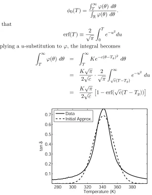
The apparent strong correlation between the process of glass transition and the tanδcurve in glassy thermoset polymers is impossible to ignore. With its peak roughly cen-tered in the glass transition region and with a width that roughly spans the glass transition temperature range, useful information can be extracted from the tan δ curve.

To help draw on the correlation assumption, it is helpful to state some essential preliminaries regarding tanδ. Tanδ is defined to be the ratio of the storage modulus (E00₎

to the loss modulus (E0_{). The storage and loss moduli are found by applying an oscillatory}

strain, defined as

ε(t) =ε0sin(ωt)

where ε0 is the magnitude of the applied strain and ω is the period of strain oscillation.

The associated stress is defined to be

σ(t) =σ0sin(ωt+δ)

where σ0 is the magnitude of the stress, ω is the same period as the applied strain, and δ

quantifies the phase lag in the stress response. The storage and loss moduli are then defined to be

E0= σ0 ε0

cosδ, E00= σ0

ε0

sinδ.

Asδ tends towards 0, the material exhibits a more elastic response since the stress response to the strain are closely in-phase, so the storage modulus,E0_{, represents the elastic/stored}

portion. Conversely, as δ tends towardsπ/2, the material exhibits a more viscous response since the stress response approaches a complete out-of-phase shift, so the loss modulus, E00_{, represents the viscous/dissipative portion. The tan δ curve (E}00_/E0_{) represents the}

viscoelastic propensity of the polymer. Many experimentalists consider the peak of the curve to be the glass transition temperature,Tg.