NE213 Scintillator Characterization Using n/gamma Digital Pulse Shape Discrimination

(1)

Abstract

LI, ANDY ON YAU. NE213 Scintillator Characterization using n/γ Digital Pulse Shape Discrimination. (Under the direction of Ayman I. Hawari.)

NE213 scintillation detectors are excellent tools for use in a mixed gamma and

neutron field due to its established pulse shape discrimination ability. With proper pulse

shape discrimination, gamma or neutron responses may be obtained in a mixed radiation

field. The neutron response needs to be deconvolved from the detector response function to

obtain an energy spectrum. To perform unfolding of neutron spectra, mono-energetic

responses are needed and the responses may be obtained via experiment or simulation of the

NE213 detector.

In this work, response functions were tested with the unfolding of a Cf252 spectrum.

Particularly, experiments were performed at the Los Alamos National Laboratory where

Cf252 spectra were obtained. During the experiment, different pre-amplifier set-ups were

tested. Namely, the pulse shape discrimination ability of the system using 50 ohm, 500 ohm,

and 1000 ohm termination resistors were compared. However, linear system responses were

not observed with the different settings. Thus, the Amoeba Simplex fitting routine was used

to augment the fall time pulse shape discrimination technique to separate the neutron and the

gamma signals. Furthermore, a new figure of merit scheme was explored to quantify the

pulse shape discrimination ability of the said non-linear system. Alongside the Cf252 spectra

experimental measurements, the program Scinful was used to generate mono-energetic

neutron responses needed for unfolding. Consequently, both the Cf252 neutron spectra and

(2)

Among the different termination resistors compared with the new figure of merit

scheme, the 50 ohm resistor setting was observed to be superior. The resultant unfolded

spectrum using the 50 ohm termination resistor shows excellent agreement between 2-10

MeV. However, even with the Amoeba Simplex method, results below 2 MeV are not

accurate due to the poor pulse shape discrimination limit of the system used. Results above

(3)

NE213 Scintillator Characterization

using n/γ Digital Pulse Shape

Discrimination

By

Andy On Yau Li

A thesis submitted to the Graduate Faculty of North Carolina State University

in partial fulfillment of the requirements for the Degree

of Master of Science

Nuclear Engineering

Raleigh, North Carolina

2007

Approved by:

_____________________ ______________________ Man-Sung Yim Wenbin Lu

______________________ _______________________ Mark Nelson Ayman I. Hawari

(4)

Dedication

This work is dedicated to Gap Tai and Loi Yau Li,

(5)

Biography

Andy Li was born On Yau Li to Wai Lun Li and Wai Ling Wu in the morning of June

14th 1984 in Hong Kong, China. He grew up in the small town of Taipo with his parents and

extended family. On Yau showed interests in math, science and literature in school and was

an avid player of Chinese flute and Chinese chess when out of class. On November 1996,

after his graduation from primary school at age 12, On Yau moved with his parents to the

United States.

On his move to the United States, On Yau changed his name for the more

Americanized name Andy. Andy and his family first moved to the small town of Morehead

City, NC, where his family owned and operated a Chinese restaurant. The restaurant

business did not last, however, and they soon moved to the North Carolina capital, Raleigh,

on January 1999. It was in Raleigh that Andy graduated from Leesville Road High School in

2002 and proceeded to enter North Carolina State University. Andy majored in Nuclear

Engineering while in North Carolina State University. At the suggestion of his adviser, Dr.

Ayman Hawari, Andy spent a summer interning out at Los Alamos National Laboratory.

While at LANL, Andy began to work on scintillation detector related project under Dr. Mark

Nelson. Andy graduated from Nuclear Engineering at North Carolina State University in

2005. He then entered the Master’s degree program at North Carolina State University

working on a joint project with Dr. Mark Nelson. Andy Plans to pursue his Ph. D. in North

(6)

Acknowledgements

First and foremost, I would like to express my most sincere gratitude to Dr. Ayman

Hawari for his guidance and direction throughout the years. I am grateful for the

opportunities he had presented to me, and I appreciate all of the efforts he had spent on my

behalf on this project. I look forward to our continued relationship for years to come.

I am grateful for the Advance Nuclear Technology group at Los Alamos National

Laboratory for hosting me. I would also like to thank Dr. Mark Nelson for working with me

in this project. Furthermore, I would like to thank Scott Gardner and Ken Butterfield for

directing my attention to Amoeba and answering my many questions about data fitting. I am

also grateful for the many others who had worked with me at LANL.

I would also like to thank Dr. Man-Sung Yim and Dr. Wenbin Lu for serving on my

thesis committee.

Finally, I am grateful for my family and my friends for their support and

(7)

List of Tables

Table 2-1-Scinful reaction types, reaction thresholds, and references. ... 38

Table 3-1-Na22 light unit calibration results... 60

Table 3-2-Lower PSD limit. ... 60

Table 3-3-Numerical Amoeba results for 500 and 1000 ohm case. ... 64

Table 3-4-Numerical Amoeba results for 50 ohm case. ... 65

(10)

List of Figures

Figure 1-1-Simplified electron excitation schematics. ... 3

Figure 2-1-Ideal hydrogen nucleus recoil energy spectrum ... 10

Figure 2-2-Effect of carbon scattering in an organic scintillation detector ... 11

Figure 2-3-Light output vs. particle type and energy by Verbinski et al ([10])... 12

Figure 2-4- Effect of nonlinear light output on an ideal spectrum deconvolved from an ideal proton scattering energy spectrum and a differential light curve. ... 13

Figure 2-5-The effect of carbon recoil and edge effect on an energy spectrum. ... 15

Figure 2-6-Effect of finite resolution on an ideal spectrum... 16

Figure 2-7-Simple experimental scheme illustrating the data branch of the zero crossing method... 20

Figure 2-8-Example of a gamma ray pulse taken with the charge integrating method. ... 22

Figure 2-9-A sample PSD histogram showing the relevant parameters for FOM calculation. ... 23

Figure 2-10-PSD histogram of a non-linear system. ... 24

Figure 2-11-PSD plot of a non-linear system. ... 24

Figure 2-12-Reflection in a 2-D case... 27

Figure 2-13-Expansion in a 2-D case... 27

Figure 2-14-Contraction in a 2-D case... 28

Figure 2-15-Shrinkage in a 2-D case. ... 29

Figure 2-16-A non-linear PSD plot obtained from Acqris digitizer with a 500 ohm termination set-up. ... 29

Figure 2-17-500 ohm PSD plot fitted with separate regressions for separation and mid-line functions... 30

Figure 2-18-Amoeba solution to the 500 ohm PSD... 31

Figure 2-19-Scinful cross section comparison with ENDF data ... 39

Figure 2-20-Carbon elastic cross-section... 39

Figure 2-21-Hydrogen elastic scattering cross-section dominates total cross-section data.... 40

Figure 2-22-Sample Scinful output with different components. ... 44

Figure 2-23-Verbinski's Curve fitted with a power function... 45

Figure 2-24-An example of a response surface for a NE213 scintillation detector... 47

Figure 2-25-Example Foreground Input File... 49

Figure 2-26-FERD's differential output for 64 bin, 50 ohm terminated Cf252 spectrum. .... 50

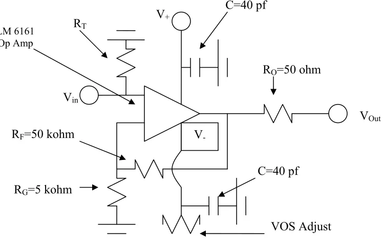
Figure 3-1-Laboratory experimental set-up used for Cf252 spectrum measurements in spring 2007... 52

Figure 3-2-Non-inverting pre-amp used with Spring 2007 set-up... 53

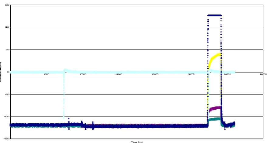
Figure 3-3-Sample pulse recorded by the Acqiris system ... 54

Figure 3-4-Sample unsaturated processed Acqiris pulse... 55

Figure 3-5-50 ohm termination fall time PSD plot... 57

(11)

Figure 3-9-Na22 spectrum taken with 500 ohm termination... 59

Figure 3-10-Na22 spectrum taken with 1000 ohm termination... 59

Figure 3-11-50 ohm light unit PSD plot. ... 61

Figure 3-16-50 ohm PSD plot... 64

Figure 3-17-Amoeba results for 50 ohm PSD. ... 66

Figure 3-18-Sample Scinful response function for 20.55 MeV mono-energetic neutron source with 3x3 NE213 detector. ... 68

Figure 3-19-Sample Scinful response function for 1.51 MeV mono-energetic neutron source with 3x3 NE213 detector. ... 69

Figure 3-20-PSD Plot of 50 ohm termination neutron data... 69

Figure 3-21-Cf252 neutron Spectrum for 50 ohm termination... 70

Figure 3-22-Ferd unfolded Cf252 spectrum for 50 ohm termination... 70

Figure 3-23-Calculated Cf252 spectrum... 71

Figure 3-24-Comparison of calculated Cf252 spectrum with the FERD unfolded spectrum..72

Figure 3-25-Cf252 500 ohm PSD neutron spectrum. ... 73

Figure 3-26-Cf252 500 ohm termination neutron spectrum. ... 73

Figure 3-27-500 ohm termination Cf252 neutron unfolded compared with calculated spectrum... 74

Figure 3-28-Cf252 1000 ohm PSD neutron spectrum. ... 75

Figure 3-29-Cf252 1000 ohm termination neutron spectrum. ... 75

Figure 3-30-1000 ohm termination Cf252 neutron unfolded compared with calculated spectrum... 76

Figure C-1-Non-inverting pre-amp used with Spring 2007 set-up, where RT is the termination resistor... 107

Figure C-2--inverting pre-amp used with Spring 2007 set-up section view... 107

(12)

Introduction

1.1 Scintillation Detectors Overview

Scintillation detectors are among the first types of detectors used for radiation

detection and measurement. Scintillation detectors detect radiation types and strength

through light emissions (scintillation) inside the detector, which is then detected and

amplified by a photomultiplier for subsequent signal processing. There are many different

types of scintillation detectors available, and each detector type possesses different

characteristics making it suitable for different purposes.

Inorganic scintillation detectors are typically crystals of alkali metals, such as

NaI(Tl), LiI(Eu), CsI(Tl) and CaI(Na), where the elements in parentheses are impurities

introduced into the crystal lattice deliberately to act as activators for scintillation. Inorganic

scintillation detectors are typically used for gamma detection due to their high counting

efficiency, which is due primarily to their high density in comparison to other gaseous

detectors. When radiation enters the detector, electrons are excited from the valence band to

the conduction band in the crystal lattice. As electrons are excited to conduction band, holes

are formed in valence band. Both electrons and holes then, commonly called electron-hole

pairs, may move around freely in the crystal lattice in the corresponding band. The amount

of electron-hole pairs are proportional to the energy deposited by the incoming radiation.

The holes drift and ionize the activator atoms, followed by the deionization of an election

capture forming a neutral configuration that may corresponds to an excited energy state of

(13)

then de-excite by emitting a photon, the photon is then amplified through the

photo-multiplying tube and a signal is generated.

In comparison to inorganic scintillation detectors which depend on the crystal

lattice’s energy bands for light generation, organic scintillation detectors depend on the

energy transition in the energy levels of a single molecule. Many organic scintillation

detectors are either liquid or plastic and are made up of mostly hydrogen and carbon, with the

most commonly used organic scintillation detectors being NE213 and NE110. As radiation

enters the detector, it interacts and excites electrons of a molecule to an excited singlet state

(denote by S1, S2, S3 where the ground state is S0). If the electron possesses energy

corresponding to a level between two states, the electron will de-excite to the lower energy

state through vibration and energy transfers to nearby electrons. Then, the electron would

further de-excite itself by scintillation (Figure 0-1). The amount of energy lost by the

electron, however, is generally less than the excitation energy to one of the energy states. As

the electron would normally de-excite to one of the sub-levels (levels between S0 and S1) of

ground state, thus preventing self-absorption, and lose the rest of its energy through

vibrations. Besides excitation to the singlet ground state where electron de-excitation

through scintillation is relatively fast, the electrons may also be excited to a triplet state,

where scintillation de-excitation is delayed. The de-excitation time for a singlet electron is in

the order of nanoseconds, where as the de-excitation time for a triplet electron is in the order

of milliseconds. Thus, excitation to the triplet state may contribute to the uncertainty in fast

measurements using an organic scintillation detector. Impurities in the scintillation may

(14)

of the radiation detected due to other mechanisms of energy loss such as heat. As in the case

of an inorganic scintillation detector, the light is then collected and amplified in the

photo-multiplying tube and a signal is then generated.

Figure 0-1-Simplified electron excitation schematics.

Both inorganic and organic scintillators rely on electron excitation and de-excitation

to generate a photon, however, each type is used in different situations. Inorganic

scintillators are typically denser than organic scintillation detectors, making their counting

efficiency higher. Also, inorganic scintillators excel at gamma detection through the

photoelectric effect due to the high Z number (atomic number) of the crystal. However,

because of their high Z number, inorganic scintillators are insensitive to high energy neutrons

as elastic neutron scattering events with high Z nuclei do not deposit much energy. Inorganic

scintillation detectors may detect thermal neutrons through nuclear reactions, such as the

6_{Li(n,alpha) reaction in the LiI(Eu) detector. For certain crystal types, the growth and}

manufacturing of a large crystal often prove difficult, which effectively limits the usage of

certain detector types to small scale laboratory applications. Organic scintillation detectors

are generally less dense, making their efficiency less than desirable. Due to the their low Z Valence Band

Conduction Band

Incoming Radiation

(15)

number, organic scintillation detectors are also not sensitive to gamma radiation except

through Compton scattering, where the gamma radiation does not deposit all of its energy in

the detector and only a continuum with energies lower than the gamma ray’s full energy is

typically observed in a gamma ray spectrum. Organic scintillators may, in comparison to

inorganic detector, detect and measure neutron energies. Since neutrons generate recoiling

nuclei in the detector with energy, depending on target mass, from zero up to potentially the

incoming energy, deducing the measured neutron spectrum requires unfolding using known

response functions. Also, with energy higher than fission neutrons (> 10 MeV), competing

carbon reactions may skew the energy spectrum and causes complications in unfolding.

Gamma ray radiations are generally present with a neutron source and may further

complicate the unfolding process. With pulse shape discrimination, the gamma rays may be

differentiated from neutrons and removed from the neutron pulse height spectrum prior to

unfolding. Compared to inorganic scintillators, organic scintillators are much easier to

manufacture. Many sizes and shapes may be made, which makes organic scintillators very

attractive for large scale neutron detection projects.

Depending on the purpose of the experiment, different types of scintillators may be

used. Inorganic scintillators are mostly used for gamma ray measurements while organic

scintillators are mostly used for neutron measurements, though organic scintillators also

require prior measured response functions to unfold the measured energy spectrum. ([1], [2],

[3])

1.2 Pulse Shape Discrimination Overview

(16)

on the measurement desired, however, some of the incoming radiation should be rejected.

Pulse shape discrimination (PSD) techniques are used to separate two or more types of

radiation and one of the main strengths of an organic liquid scintillator is its ability to

perform PSD in a mixed radiation environment. Traditionally PSD performed on

scintillators is based on several principles. First, it is well known that different particles have

a different associated stopping power in a medium and tt follows then that different particles

interact differently in a medium. Mainly the heavier particles (such as alphas), which have a

high stopping power, are observed to produce a quenching effect, resulting in less light being

produced per particle’s incoming energy. Quenching causes the excited electrons to

de-excite via radiationless processes, such as phonen and heat. Conversely the lighter particles

(such as electrons) quench less, resulting in effectively a higher amount of light being

produced in comparison with a heavy particle of equivalent energy. Some PSD techniques,

such as the rise time technique which is common in gas detectors, are based off of the direct

consequence of the clustering of charges on heavier particles (Also called quenching in gas

detectors), while other PSD techniques are based upon the decay fluorescence of the

scintillator. As stated, heavier particles tend to quench the detector volume resulting in a less

light being procuded overall in comparison with lighter particles. Heavier particles also

generate more triplet electrons than lighter particles. Normally electrons excite to a singlet

excitation state, but more triplet states can be observed with heavy incoming particles.

Triplet states have a longer de-excitation time than singlet states, thus resulting in longer

decay fluorescence time for the scintillator. Some PSD techniques, such as the fall time and

the charge integration techniques are based upon the decay fluorescence difference of the

(17)

Over the years, the aforementioned techniques were explored and used with success,

and they will be described in details a later section. With the advent of computers and data

analysis tools, the recent efforts in developing PSD had shifted from hardware focused

approaches (such as the Forte method and other analog methods ( [5], [6]), which will be

described) to data analysis approaches (such as statistical estimates and template matching

technique ([7], [8], [9])). Specifically, the later approach performs PSD on mixed

particle-type data post data collection rather than performing PSD during data collection. This

approach allows for flexibility in the development and the implementation of the PSD

technique to the data obtained. However, this approach is also often more time consuming

and requires more data storage space than concurrent data collection PSD. In this work, a

post data collection PSD technique using the amoeba simplex regression is explored and

(18)

Chapter 2 Liquid Scintillator Detection Principles

2.1 Proton Recoil Mechanisms

In an organic scintillator, proton recoil occurs when an incoming neutron collides

elastically with a proton. The proton then ionizes surrounding electrons in its track for

subsequent detection. Since a neutron has the approximately the same mass as a proton, the

neutron may transfer all of its energy to a proton in one collision depending on the angle of

collision. Therefore, a precise response function of the detector must be known to unfold the

resulting proton continuum. Besides proton collisions, a neutron may also collide with

carbon atoms in the detector, causing a skew in the resulting spectrum.

Assuming stationary proton in the laboratory system, neutrons and protons with

non-relativistic energy (E<<939 MeV) have energies Enc and EPc in the center of mass system

where n P n P c n E m m m

E ₍ ₎2

+

= 2.1

n P n P n c P E m m m m E ₂ ) ( +

= 2.2

En is neutron energy in the laboratory system; mn and mP are mass of the neutron and proton

respectively. With Q=0 in neutron scattering, the products Enc’ and EPc’ have the same total

energy as the reactant. Also, in atomic mass units, neutron has a weight of 1 and proton has a

weight of A and thus Equation (2.1) and (2.2) maybe rewritten as

n c

n _A E

A E

E ₎2

1 ( '

+ =

(19)

n c P c P E A A E E ₂ ) 1 ( ' + =

= 2.4

Upon conversion from the center of mass system into the laboratory system, the recoiled

proton energy EP becomes

n

P E

A A

E (1 cos )

) 1 (

4

2 − α

+

= 2.5

where α is the neutron scattering angle in the center of mass frame. Upon transformation of

α toϑ, whereϑis the recoil angle measured from the incoming neutron’s initial path in the

laboratory frame, Equation (2.5) becomes

n

P E

A A

E (cos )

) 1 ( 4 2 2 ϑ +

= 2.6

Since A and En are constant for a given interaction, the maximum and minimum of

the recoil proton’s energy then depends on the scattering angle. The minimum energy is zero

and it occurs when the recoiled proton scattered perpendicularly from the neutron. The

maximum energy of the recoiled proton is

n P E A A E ₂ ) 1 ( 4 +

= 2.7

which occurs when the proton is forwardly scattered.

Since a continuum from zero energy up to energy shown in Equation (2.7) is

expected, the probability of interaction for each scattering angle must be examined to

estimate the shape of the ideal spectrum. Let P(α)dαbe the probability that a neutron will

(20)

s d d P σ α σ α α π α

α) 2 sin ( )

( = 2.8

where 2πsinαdα is the differential slice of an angle dα aboutα to all space, and s

σ α σ( )

is

the fraction of neutrons scattering into the angleα . If P(E_P)dE_Pis defined as the probability

of a neutron that will be scattered into an energy dE_P aboutE_P, where the recoiled energy

P

E is caused by scattering angleα, then

P P dE

E P d

P(α) α = ( ) 2.9

and s P P P dE d dE d P E P σ α σ α α π α

α) 2 sin ( )

( )

( = = 2.10

Using Equation (2.5) to substitute the relationship P

dE dα

, Equation (2.10) becomes

n s P P E A A dE d P E P π σ α σ α

α) (1 ) ( )

( ) ( 2 + =

= 2.11

In the case of a hydrogen atom, neutron hydrogen scattering is isotropic up to about

14 MeV. Thus, substituting

π σ α σ 4 )

( ₌ s _{into Equation (2.11) and}_A_{=1 for hydrogen, it}

becomes

n P

E E

P( )= 1 2.12

As can be seen with Equation (2.12), for an ideal hydrogen scattering detector, the ideal

energy spectrum is simply a uniformly distributed continuum between zero energy and initial

(21)

Figure 2-1-Ideal hydrogen nucleus recoil energy spectrum

In Figure 2-1 above, an ideal hydrogen nucleus recoil energy spectrum is shown,

where the probability for a neutron interacting in the detector volume is equal for all

energies. In a real detector, however, many different factors contribute to the formation of

the measured spectrum. The many factors which contribute into a real spectrum will be now

discussed ([1], [2], [3]).

2.2 Spectrum Distortions

2.2.1 Carbon Scattering

All organic scintillation detectors contain carbon. From Equation (2.7) it can be seen

that the maximum amount of energy transfer from a neutron to a carbon in a single collision

is 28% of its initial energy. Combined with the low light output from heavy particles

(Non-linearity of light output will be explained in a later section), scattering from carbon alone

only contribute to low energy events and will cause a skew in the spectrum favoring low

energy events (Figure 2-2).

En Ep

1/En

(22)

Furthermore, the carbon scattered neutron may scatter again with another proton in

the detector volume. Since the neutron will have lower energy after initial scattering with the

carbon nucleus, the neutron may at most deposit 72% of its initial energy in its second

scattering (assuming with a hydrogen atom). Therefore, fewer events will be recorded in the

resulting energy spectrum corresponded to energy between 72% to 100% of the maximum

neutron energy due to carbon scattering ([1], [2]).

Figure 2-2-Effect of carbon scattering in an organic scintillation detector

2.2.2 Nonlinear Light Output

Depending on the energy and the particle type incoming or recoiling in case of

neutron detection, the light output of an organic scintillation detector may not be linearly

proportional to the incoming radiation’s energy. The reason for the nonlinearity of light

outcome is unknown, but is suspected to be the result of nonlinear specific energy loss by

heavy charge particles inside the detector. Specifically, gamma rays and electrons exhibit

linear responses, while protons and neutrons exhibit nonlinear light output ([1], [2],[10]).

En Ep

1/En

dN/dE

(23)

For example, Figure 2-3 illustrates the characteristic light output of a NE213 detector as a

function of particle energy.

0.001 0.01 0.1 1 10 100

0.1 1 10 100

Energy (MeV)

Li

gh

t O

ut

pu

t

Proton (A=1) Alpha (A=4) Carbon (A=12)

Figure 2-3-Light output vs. particle type and energy by Verbinski et al ([10]). The proton light output is related to energy byL=1.13E_R1.4318.

For hydrogen atoms, the light output L from proton recoil is approximately related to

energy E_Rby

2

3

R

kE

L= 2.13

where k is a proportionality constant.

Spectra obtained from an organic scintillation detector are typically calibrated to give

the quantity

dL dN

, or number of counts in a bin with widthdL. To obtain the energy

spectrum

dE dN

, the light spectrum must be transformed with the quantity

dE dL

(24)

dE dL dL dN dE dN ₌ 2.14 where dE dL

may be obtained from Equation (2.13)

2 1 2 3 R kE dE dL

= 2.15

Moreover, with Equation (2.13), (2.14) and (2.15), it can be shown that the shape of

the light spectrum

dL dN

obtained is skewed by the quantity

dE dL

(Figure 2-4, [1]), where

3 1 2 1 ' 2 3 Constant − = =

= k L

kE dE dL dE dN dL dN R 2.16

where k’ is simply a proportionality constant.

Figure 2-4- Effect of nonlinear light output on an ideal spectrum deconvolved from an ideal proton scattering energy spectrum and a differential light curve.

dN/dE

E

E dH/dE ≈ 3/2kE1/2 dH/dE

dN/dE

(25)

Also as can be seen in Equation (2.14), the quantity

dE dL

must be known accurately to

determine the energy spectrum. Since the energy spectrum

dE dN

must be unfolded to obtain

the source spectrum, an error in

dE dL

would be compounded in the final source spectrum. For

the purpose of obtaining the energy spectrum, the curves presented by Verbinski et al.

(Figure 2-3, [10]) will be used.

2.2.3 Light Calibration

Since a NE213 detector does not output in energy or light unit directly, a light

calibration must be made. One light unit in a detector for a given gain setting is defined as

1.13 times the half height of the Na22 1275 keV energy peak ([6]). Thus, any spectrum

taken with the NE213 detector should be taken with a Na22 spectrum as well to calibrate the

results to light or energy scale.

2.2.4 Edge Effect

If the incoming neutrons have sufficient energy such that the recoiled proton’s mean

free path is not small in comparison with the detector dimensions, then edge effect will be

observed in the detector output. Edge effect is caused by incomplete energy deposition by

the recoiled protons. The protons, after recoil, will deposition some of their energy through

electron ionization then escape the detector volume. Thus, the resulting energy spectrum of

(26)

Figure 2-5-The effect of carbon recoil and edge effect on an energy spectrum.

2.2.5 Multiple Hydrogen Scattering

For large detectors, it is possible for neutrons to undergo multiple scattering before

stopping or escaping from the detector volume. If a neutron undergoes multiple carbon

scatterings, then the resulting spectrum would be similar to that resulting from a single

carbon event, where more low energy events will be observed. On the other hand, if the

neutron undergoes multiple hydrogen scatterings, the effect could be significant in the

resulting spectrum. All events from a single neutron, even from multiple scatterings, happen

within a short period of time and will be recorded as one even in the final spectrum. Since

the average energy lost in a single neutron hydrogen collision is half of the neutron’s initial

energy, multiple scatterings with hydrogen increases the energy transferred to the detector

and causes more high energy events to be observed. Counts

E

Heavy-atom Recoils

Wall and end effects

(27)

2.2.6 Finite Detector Resolution

Since no detector possesses perfect resolution, the energy spectrum obtained will

always be smeared in comparison with the ideal spectrum (Figure 2-1). In essence,

electronic noises, non-uniform light collection (Due to the difference in the location of

interaction), and the statistical nature of detection techniques all contribute to the finite

resolution of the detector as shown in Figure 2-6 ([1]).

Figure 2-6-Effect of finite resolution on an ideal spectrum.

2.2.7 Pulse Shape Discrimination Capability

Liquid scintillators are capable of detecting both neutron and gamma pulses.

Neutrons mostly react through isotropic proton recoil as described. Gamma rays, due to the

low-z (atomic number) content of the scintillator, generally react through Compton scattering

as oppose to photoelectric events in other gamma detectors. Furthermore, different particle

type causes electron excitation through different excitation mechanisms. Since neutrons

react mainly through proton recoil, the ionization density along the recoiled proton’s track is

high enough to produce triplet state electrons and thus producing high decay fluorescence. In

dN/dE

E

(28)

contrast, gamma ray reactions mainly produce singlet state electrons and lower decay

fluorescence. Specifically, the light produced from the NE213 scintillator has three distinct

components: a short 3 ns rise time, an intermediate 32 ns transient and a long 270 ns fall time

which is affected by the decay fluorescence ([4]). Pulse shape discrimination (PSD) for

NE213 detectors typically makes use of the 270 ns tail component to distinguish between

neutrons and gammas. The PSD ability is important with measurements taken in a mixed

gamma/neutron area where only one particle’s response is desired, PSD can filter out the

undesirable particles’ responses from the detector.

2.3 Pulse Shape Discrimination Methods

The ability of the NE213 scintillator to perform PSD is extremely important as it allos

for the separation of signals in a mixed field environment. For example, most neutron

measurements have gamma back ground signals, with PSD, the gamma signals may be

filtered. PSD techniques are used to separate two or more types of radiation. Over the years,

several PSD methods were proposed and implemented for different scenarios and they each

have their strengths and weaknesses. This section will give a brief introduction to some of

the methods that had been used in recent years.

2.3.1 Rise Time Method

Proportional counters often use the rise time method (RT) to perform PSD in a mixed

environment. In organic scintillators, different particle types cause a difference in the decay

light component, whereas in gas-filled proportional counters, a difference in the rise time is

(29)

Heavy particles in a proportional counter typically have a much shorter range than

light particles, thus the ionization track of the heavy particles is much shorter than that of the

lighter particles. An example is that gamma rays induced fast electrons often will pass

through the proportional counter where as a neutron recoiled proton will follow a short path

and comes to rest within the detector volume. It follows that the shorter track of the heavier

particles has a shorter corresponding charge collection time compared with the longer track

of the lighter particles. The difference in rise time may then be exploited to perform PSD

([1]). Since liquid scintiallors de-excite through a different mechanism, the rise-time

difference is not directly observed ([1], [2]). However, liquid scintillators may use a

preamplifier with a time constant to integrate the fall time of the pulses, and thus imitate the

rise time method. With the RT method in general, a rise time to pulse height converter

(RHC) can be used to convert the rise time to a pulse. The magnitude of the resulting pulse

then is indicative of the pulse’s particle type. A single channel analyzer then may be used in

conjunction with a coincident counting system to filter out a certain type of particles. The

strength of this particular method is its accuracy: 1/500 false rejection for neutron with

energy less than 500 keV and 1/50 for neutron with energy less than 60 keV ([6]). The

limitation of this method is its dependency on the hardware and the restriction of gas

proportional counters.

2.3.2 Forte Method

The Forte method is a PSD scheme used with a pulse shape discriminator designed by

Forte. The circuitry uses signals from the anode and some of the dynodes in the

(30)

or large negative pulse for gammas ([2]). The signals may then be gated with coincidence

modules and delay lines to achieve PSD. The main strength of this method is the type of

pulses created making neutron and gamma pulses easily distinguishable once the original

pulse passed through the PSD circuitry. The main draw back for the Forte method is that it is

extremely hardware intensive. The dynodes used must be tested with the correct gain to

ensure no saturation occurred, and then modifications of the photomultiplier tube base must

be done so then the dynode may output the correct signal to the pulse shape discriminator.

Also, the Forte method must be used with the correct pulse shape discriminator (designed by

Forte). Even though this method is not usable for those who do not possess the hardware

described, its description here serves as an illustration on the variety of PSD schemes and the

various in-house designed hardware which may accompany them ([5], [6])

2.3.3 Zero Crossing Method

The zero crossing method (ZC) utilizes the zero crossing point of the pulse as a

reference to perform PSD. The zero crossing point is the point at which a bipolar duplication

of the original pulse, made by super-imposing an inversion of the original pulse, crosses the

zero bias axis. The ZC scheme first separates the signals into multiple branches (Figure 2-7).

The scheme then uses either a double delay line or a CR circuit to help find the zero crossing

point of a given pulse. The interval between the zero crossing point and the leading edge of

the pulse gives an indication of the fall time of the pulse, and thus pulse shape. The time

difference is fed into a time to amplitude converter and then the gamma and neutron signals

are separated by the discrimination setting on a single channel analyzer down in the data

(31)

main advantage of this method is its sensitivity to low energy pulses, which is effective down

to about 30 keV neutrons with the use of a time of flight scheme concurrently. However, a

constant fraction discriminator along with a time to amplitude converter must be used with

this scheme. Several reports compared this method favorably with the charge integration

method ([10]).

Figure 2-7-Simple experimental scheme illustrating the data branch of the zero crossing method.

2.3.4 Fall Time Method

The fall time method utilizes the same principle as the ZC method, in that the fall

time of the pulses examined is indicative of the pulse shape. The difference between the two

methods, however, is that the fall time method measures fall time directly, whereas the ZC

method measures the fall time through a series of analog time gates. The fall time may be

measured with analog equipment or with post-data collection analysis. Since neutron pulses

have higher decay fluorescence, their fall time will be higher than gamma pulses. The main NE213

Detector Anode Buffer Preamplifier

Pulse Shape Analyzer

Amplifier Time to Amplitude

Converter (TAC)/Single Channel Analyzer

(SCA) Multi Channel

Analyzer (MCA) _Delay

Neutron Pulse Height Spectrum

(32)

advantage of this method is its flexibility in that the fall time may be measured during or

after data collection. However, with some setups, the fall time is not as stable as the ZC

method. The fall time reference may drift with differing pulse size, leading to non-ideal PSD

spectra.

2.3.5 Charge Integration Method

The charge integration method (CI) is the least hardware intensive method out of all

schemes mentioned. CI compares a short portion of the pulse’s charge with its total charge,

the tail-to-total ratio or the rise to total ratio, to determine the pulse shape. An example of an

integrated gamma pulse is shown in Figure 2-8. The ratio used depends on the detector used;

the tail ratio is normally used with liquid scintillators and the rise time ratio with gas

detectors. Gammas and neutrons are separated by a tail-to-total ratio specific to the system

used; the ratio may be used post data-collection to perform PSD. In principle, this method is

similar to ZC, with the exception that the difference between the gamma and the neutron

pulses is compared on a normalized basis. Though several papers had pointed out that with

lower incoming particle energies, ZC is superior to CI. The main strength of CI, however, is

that CI is relatively straight forward to implement. In principle, only the detector and a

digitizer are needed to record the pulse shape. In actuality, however, the pulses may have to

be shaped and conditioned before recording so a few other components such as a

pre-amplifier may be desired. Even with the added components for pulse shaping, the CI system

is much simpler than other PSD systems mentioned. Also since PSD maybe performed by

software, more flexibility is allowed in the data collection components and implementation

(33)

Figure 2-8-Example of a gamma ray pulse taken with the charge integrating method.

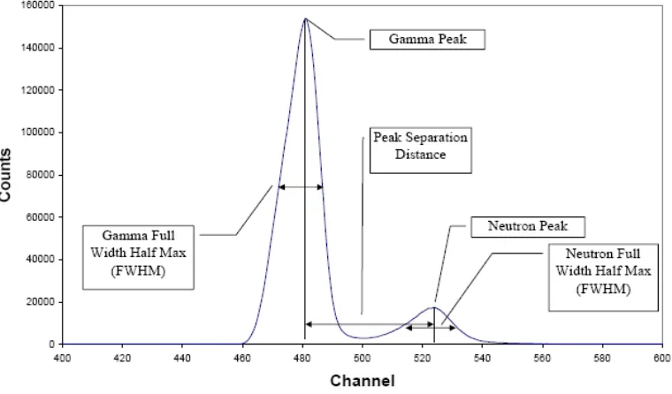
2.4 Figure of Merit

NE213 liquid scintillation detectors’ ability to perform PSD enables it to be employed

in a neutron/gamma mixed field. The figure of merit (FOM) is a measure of a detector

system’s PSD capability and may be given by

) (

FOM

n

FWHM FWHM

s

+ ∆ =

γ

2.17

Where ∆s is the separation between the gamma and the neutron peak, and FWHM is the full

width at half max of the individual peaks. The peaks described are the individual particle’s

peak seen in the histogram of the PSD parameter (Figure 2-9). A good PSD capability is

denoted by a large FOM value. As a large FOM value consists of a large peak separation

(34)

Figure 2-9-A sample PSD histogram showing the relevant parameters for FOM calculation.

Typically, PSD results are plotted in such a way that the FOM capability of the

system can be easily visualized. Specifically, there are two common types of PSD plots: one

with the PSD parameter plotted against a normalization parameter and one is a histogram

representation of the PSD parameter. For the histogram type the PSD parameter is shown

explicitly after binning ([1], [2]).

A problem with the aforementioned FOM scheme is that the scheme only takes into

account a linear spectrum. If non-linearity exists in the system, then more than two peaks

may be observed (Figure 2-10). In such cases, the definition of FWHM for the neutron and

the gamma peaks becomes unclear, and another scheme should be used.

2.5 Modified Figure of Merit

When non-linearity exists in the system or when the traditional FOM scheme is not

(35)

PSD capability of the system ([15]). In the PSD histogram below, due to non-linearity of the

system gain, multiple peaks exist. In such cases, the traditional FOM scheme breaks down as

the definition of the peak separation and the FWHM becomes unclear.

Figure 2-10-PSD histogram of a non-linear system.

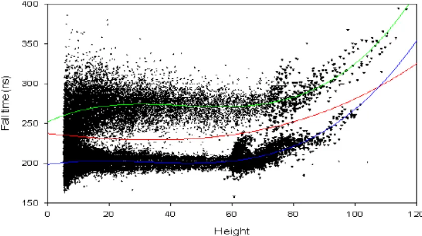
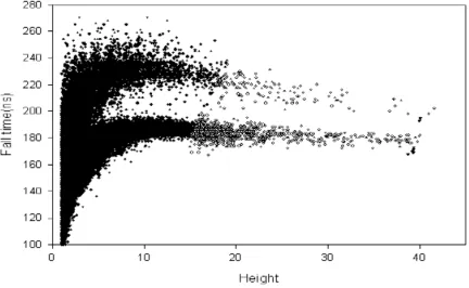
The corresponding PSD scatter plot of the Figure 2-10 is below in Figure 2-11. In the

scatter plot, it is clear that the fall time of the pulses does not vary linearly with the height of

the pulse. Furthermore, it is clear that the peaks of Figure 2-10 are created from the

curvature of the scatterplot.

(36)

In Figure 2-11, a separation function (Red line), a neutron mid-line (Green line) and a

gamma mid-line (Blue line) function are plotted. With the functions, a new FOM scheme

(FOM*) may be derived with the following expression:

)) ( ) ( ( ) ( ) ( * FOM n dh dh h h n σ γ σ γ + − =

∫

2.18

The numerator expression

∫ ∫ − dh dh h h

n( ) γ ( ) _{describes the neutron and gamma peak}

separation by normalizing the difference between a neutron and a gamma mid-line function

represented by n(h)andγ(h)as shown in the PSD plot. Furthermore, the denominator term

(

σ(γ)+σ(n)

)

described the combined spread of the peaks. σ(γ)is the standard deviation of

the gamma peak in respect to the gamma mid-line function and σ(n)is the standard

deviation of the neutron peak. As can be seen, the new FOM scheme preserves the definition

of the traditional FOM scheme by using translated expression for both the numerator and the

denominator terms. Furthermore, if an appropriate fitting routine is used to calculate the

separation and the mid-line functions, a more objective FOM may be obtained, as the new

scheme’s definitions are more clear than the old scheme’s, especially when in the old FOM

scheme the FWHM of the peaks are not readily clear when the peak separation is small.

**2.6 FOM* Function Fitting**

To fit the neutron and the gamma mid-line functions separately, an initial arbitrary

separation function will need to be defined. However, all three functions may be fitted

(37)

The amoeba simplex fitting routine is also called the Nelder-Mead Simplex Method,

and was first developed by Nelder and Mead. A simplex is a generalized triangle with (n+1)

vertices in an n-dimensional plane. The method uses a sequence of simplexes to find the

minimum of a given function f(a₁,a₂,...,a_n). The amoeba algorithm is intrinsically

non-linear and is effective in bypassing local minima during minimization.

2.6.1 Amoeba Algorithm

The simplex method for finding the minima of a given function

) ,..., , ( )

(A f a₁ a₂ a_n

f = will be given in this section.

1) With an n-parameter function f(a₁,a₂,...,a_n), )(n+1 initial points must be chosen.

For example, for a 2-parameter function f(A)= f(a₁,a₂), three initial

guesses f(X)=(x₁,x₂), f(Y)=(y₁,y₂)and f(Z)=(z₁,z₂)must be chosen.

2) Define }B={b₁,b₂,...,b_n (B for best), where f(B)= f(b1,b2,...,bn) produces the

smallest function from the pool of values. Similarly, define W ={w₁,w₂,...,w_n} (W

for worst), where f(W)= f(w₁,w₂,...,w_n) produces the largest function value. The

goal now is to shrink the simplex in such a way that W improves.

3) With B and W defined, it is then possible to find the mid-point M, where M is the

average of all points excluding W. With M then, a reflection R may be found.

Specifically, R denotes the set of coordinates given by a projection of W along M,

(38)

4) If f(R)= f(r₁,r₂,...,r_n)is less than f(W), an expansion point should be tested.

Basically, the point E denotes an expansion of R along the mid-point M,

whereE =R+(R−M) (Figure 2-13).

Figure 2-12-Reflection in a 2-D case.

5) If either f(R)or f(E)is smaller thanf(W), then f(W)should be replaced by the

smallest value of the two. After the replacement, the whole process is repeated from

step 2). However, if f(W)is less than f(R), then two contraction points

1

C andC2should be considered (Figure 2-14).

Figure 2-13-Expansion in a 2-D case.

B

W

G

R M

B

W

G

R

(39)

6) The points C₁andC₂are defined as the mid-points between W-M and M-R,

respectively. Thus ( ) 2

1

1 W M

C = + and ( )

2 1

2 M R

C = + . The smaller function value

between f(C₁)and f(C₂)is then compared with f(W). If either f(C₁)or f(C₂) is

smaller than f(W), then W is replaced by the point and the process is repeated from

step 2).

7) If none of the function values f(R),f(E),f(C1)or f(C2) is smaller than f(W), the

simplex must shrink toward the best point B (Figure 2-15). Specifically, every

vertices of the simplex B,X,Y,...,Wundergoes the transformation ( ) 2

1

* X B

X = + .

Afterwards, the function f is then re-evaluated at every point and the order of

W Y X

B, , ,..., are reassigned and the process begins anew from step 2).

Figure 2-14-Contraction in a 2-D case.

8) The process repeats until a given tolerance is reached, typically defined by

(

f(B) f(W)

)

T < − .

For a more detailed explanation of the amoeba scheme, please refer to [16], [17]. B

W

G

R M

(40)

Figure 2-15-Shrinkage in a 2-D case.

2.6.2 Current Implementation

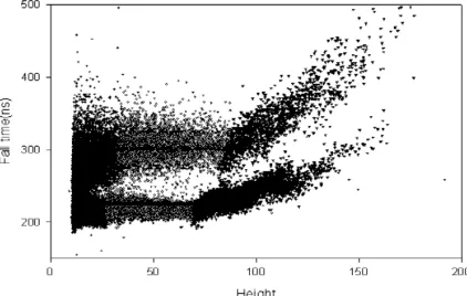
The current problem lies in fitting suitable curves to the PSD plots obtained from

non-linear system, such as Figure 2-16. The curves are needed to obtain a modified figure of

merit (FOM*), which is discussed in an earlier section.

Figure 2-16-A non-linear PSD plot obtained from Acqris digitizer with a 500 ohm termination set-up.

G W

S M

(41)

Originally, a gamma/neutron separation curve was fitted manually to the space

between the upper neutron and the lower gamma region. Then separate linear regression

lines are fitted to each of the regions. Cubic regressions were used to fit the separation and

the mid-line functions in this method. With this method, however, the separation function is

needed, and since the curve is fitted manually (Figure 2-17), huge error may be present.

Furthermore, the neutron and gamma regression lines often crossed and caused errors in

subsequent calculation. Thus, the option of using the amoeba method to fit all three curves

simultaneously was explored and tested (Figure 2-18).

The function that simplex minimizes in this case is the simple regression:

( )

(

)

∑

−

= _X _X _h 2

f _i 2.19

WhereX_iis the individual date point andX

( )

h is the fitted function of height (h).

(42)

Figure 2-18-Amoeba solution to the 500 ohm PSD. Green line is the neutron mid-line function, red the separation function and blue the gamma mid-line function.

According to Figure 2-16, there are three distinct regions in the PSD plots: the upper

neutron, lower gamma and the middle separation regions. As such, three cubic equations are

used (Figure 2-18) and referenced in the amoeba routine, and they are as follows:

( )

_h ₌_a ₊_bh₊_ch2 ₊_dh3

γ

γ 2.20

( )

_h _a _a _bh _ch2 _dh3

S = _γ + _S + + + 2.21

( )

_h _a _a _bh _ch2 _dh3

N = _γ + _N + + + 2.22

In the equations above, a_γ,a_S,a_N,b,c,dare free parameters and amoeba is free to adjust

them. A note of interest is that the three regions are assumed to be the same shape, thus the

only difference between the equations is the intercept terma. Also, the presented equations

(43)

2.6.3 PSD Implications

As shown in Figure 2-18 above, the amoeba method may be used to separate neutron

and gamma data. Even though in the current implementation, amoeba is used to obtain

functions for the FOM* scheme, the amoeba method itself is a powerful method that may be

used outside of the current scope. Even with the traditional FOM scheme, a need exists to

separate neutron and gamma data. If the detection system is set up in such a way that allows

for post data collection PSD, the amoeba method may easily be used to extract neutron data.

Even in a linear concurrent PSD-data collection system, the amoeba method may still be used

to find the optimum value of the PSD parameter, such as the lower level discriminator cut-off

in a traditional charge integrating system. The capability of amoeba performing PSD on a

non-linear post data collection PSD system will be demonstrated in the experimental section;

however, its ability to perform PSD on any system should not be overlooked.

2.7 Response Function

With good PSD techniques, neutron spectra may be separated from gamma spectra in

a mixed field measurement data set. If the neutron data set is obtained from a

mono-energetic neutron source, then the detector’s response function for that particular neutron

may be determined ([18], [19]). To illustrate, consider the probability of a recoiled proton’s

energy is in intervaldEaboutE where

dE E dE E P

n P

1 )

( = 2.23

Then the ideal proton energy spectrum with bin widthdE_P, defined to beN(E_P)dE_P, is given

(44)

∫

− = max

0 ( ) ( ) ( )

)

( E _n _P

n P n n n H P

P H E E

E dE dE E E T N dE E

N σ φ 2.24

where

H

N =Hydrogen atom number density

T=Time of measurement of the recoil protons

) (E_n

σ =Elastic scattering cross section of hydrogen

n n dE

E ) (

φ =Neutron flux of neutrons with energy dE_naboutE_n

n P

E dE

= probability of a recoiled proton’s energy is dE_PaboutE_P

) (E_n E_P

H − =Function with valueH(E_n −E_P)=1E_n ≥E_P, and 0 otherwise

The measured spectrumM(E)dE with all of the spectrum distortions taken into

consideration is given by

∫

= max

0 ( , ) ( )

)

(E dE E dER E E_P N E_P dE_P

M 2.25

dE E

M( ) may also be expressed in terms of the neutron source spectrum (or neutron flux)

n n dE

E ) (

φ , where

∫

= max

0 ( , ) ( )

)

(E E dE_nk E E_n E_n

M φ 2.26

In both Equation (2.25) and (2.26), bothR(E,E_P)andk(E,E_n)are defined as the response

function to relate the ideal neutron spectrum and the neutron flux spectrum to the measured

spectrum. k(E,E_n)can be related to R(E,E_P)through the relationship

) ( ) ( ) , ( ) , ( max

0 n P

E n n H P P

n H E E

E E T N E E R dE E E

(45)

To unfold the measured spectrum to obtain the source spectrumφ(E_n)then, both

dE E

M( ) andk(E,E_n)must be determined. M(E)dE is simply the measured spectrum,

obtainable through a detector system. k(E,E_n)can be determined by characterizing the

detector system. As can be observed through Equation (2.26), if the neutron source is

mono-energetic with energy E, Equation (2.26) may be rewritten as a differential spectrum with the

source flux φ₀

dE E E k dE E

M( ) = ( , _n)φ₀ 2.28

With the aid of an accelerator as a source for monoenergetic neutrons or a computer

simulation to simulate the source detector interaction, the response function for

mono-energetic neutrons with different energy may be determined. Then, if the quantity

) , (E E_n

k for many energy levels is known, a response surface maybe constructed for a range

of energies. The response surface may then be used to unfold the measured

spectrumM(E)dE to obtain the source spectrumφ(E_n) (Equation (2.26)). For this project,

the program Scinful (Scintillation Full Response to neutron detection) is examined and used

for the purpose of generating response functions k(E,E_n) for neutron spectrum unfolding.

2.8 Scintillator Full Response to Neutron Detection

Scinful (Scintillator Full Response to Neutron Detection) is a Monte Carlo program

which can be used to simulate NE213 or NE110 scintillation detectors. In Scinful, a

cylindrical detector and a point source are modeled; each particle from the source is

monitored and tracked through out the program. The final output from Scinful is a

(46)

spectrum, where L is the light output from the detector. Besides the total spectrum, Scinful

can also give the light output from each individual reaction, and if desired, Scinful can also

output the spectra in terms of energy instead of light output. In the following sections,

Scinful will be dissected and each process of the calculations will be discussed ([20], [21]).

2.8.1 Input File

The input file of Scinful consists of seven lines and they are given below:

1) Comment Lines

2) # of Histories, Detector Type, Attenuation Coefficient

3) Source Energy, Low Energy Bound, Distribution, Energy Cut off

4) Random Number Generator Seed

5) x, y, z of the source location

6) Detector Radius, Detector Height, Collimator Radius

7) Wbox

The interpretation of each variable:

Comment Lines- This line is designated to the description of the program, this line may be

left blank

# of Histories- Number of interaction simulated in the detector

Detector Type- May be either 213 or 110, a negative sign in front of the numbers denotes

pulse shape discrimination

Attenuation Coefficient- The attenuation coefficient for light transport in the detector, Scinful

(47)

Source Energy- The upper bound of the source energy in MeV, if the source is

mono-energetic, this is the source energy. The magnitude of the source must be less than 100 MeV.

Low Energy Bound- The lower energy bound of the source energy in MeV, 0 should be

inputted if the source is mono-energetic.

Distribution- The distribution of the source energy:

0 if the source is mono-energetic

<0 if the source energy is uniformly distributed

>0 if the source follows a Maxwellian distribution with temperature equals to the

number inputted

Random Number Generator Seed- Seed for the random number generator

x, y, z of source location- the (x, y, z) coordinates of the source. The origin of the coordinate

system is the center of the detector front face. The x, y plane is the detector front face and

the negative z axis runs along perpendicular to the front face of the detector.

Detector Radius- The radius of the detector in cm.

Detector Height- The height of the detector in cm.

Collimator Radius- The radius of the front collimator in cm.

Wbox- Scinful uses Wbox to calculate the width of light bins used in the spectrum.

2.8.2 Solid Angle Determination

Scinful determines the solid angle of the source through Monte Carlo method.

Scinful first estimates a solid angle which encompasses the entire detector surface.

Depending on the source location in respect to the detector, the method of estimation will be

(48)

closest and the furthest edge on the detector surface, the angle between the two lines is

Scinful’s first estimate of the solid angle. If the source is positioned in such a way such that

both the sides and the front face of the detector is visible to the source, Scinful calculates the

front face component and the side component separately then sums the two.

After the initial estimate is chosen, Scinful then emits particles in the estimated solid

angle. If a particle does not hit the detector surface, a new particle will be generated until the

detector surface is hit. If the detector surface is hit, Scinful will then track the particle in the

detector and perform subsequent calculations. In the end, the total number of particles

emitted and the particles hitting the detector is tallied. The final true solid angle then is

simply the initial solid angle times the ratio of the tracked particles.

2.8.3 Interaction

After the solid angle is determined, the energy of the particles emitted is sampled

from the energy distribution specified in the input file. With the energy of the particle then,

all of the cross-sections pertained to the energy are tallied. Except for hydrogen in which an

experimental fit is used, all of the other cross-sections are stored in tabular form in the

program. In all, eleven different types of interactions are taken into account in Scinful.

Table 2-1 contains the eleven reaction types in Scinful, respective reaction threshold, and the

reference for each reaction ([22]).

The hydrogen cross-section agrees extremely well with ENDF/B-V data (Figure

2-19). The carbon reaction cross-sections, on the other hand, typically agree well with

ENDF/B-V data at low energy, but deviates above 15-20 MeV (Figure 2-20). The deviation

(49)

the reactions. Furthermore, the reactions listed above with an * in the reference are not found

in ENF/B-V cross-section archive. The reliability of those cross-sections is suspicious due to

the lack of data on them, as only one or two papers had published results on those reactions.

Furthermore, only one major reaction with Hydrogen is listed, whereas ten different carbon

reactions are listed in Scinful. This is primarily due to the fact that hydrogen elastic

scattering cross-section dominates the hydrogen total cross-section for energy above 1 eV

(Figure 2-21), which is the effect range of the program due to other tabulation limits (Such as

proton range table used in range calculations).

Table 2-1-Scinful reaction types, reaction thresholds, and references.

Reaction Types Threshold Reference

(n,H) Elastic Scattering - ENDF/B-V

(n,C) Elastic Scattering - ENDF/B-V

(n,C) Inelastic Scattering 2.5 MeV ENDF/B-V

C(n,2n)B 21.5 MeV ENDF/B-V

C(n,α)Be 7.5 MeV ENDF/B-V

C(n,d)B 15.25 MeV ENDF/B-V

C(n,p)B Bounded State 13.7 MeV ENDF/B-V

C(n,p)B Unbounded State 17.35 MeV Datum*

C(n,n')3α 17.35 MeV Nuclear Physics A394*

C(n,t)B 21.5 MeV Subramamian*

(50)

Figure 2-19-Scinful cross section comparison with ENDF data, hydrogen cross-section confirms well with ENDF data.

(51)

Figure 2-21-Hydrogen elastic scattering cross-section dominates total cross-section data.

After Scinful tallies all of the available sections, the fraction of each

cross-section to the total cross cross-section is then found. A number generator then generates a number

to compare to the hydrogen fraction. If the hydrogen fraction is greater than the random

number, hydrogen elastic scattering will then occur for the particular particle. If, however,

the random number is greater than the hydrogen fraction, the random number less the

hydrogen fraction will then be compared with carbon elastic scattering. The process

continues until a reaction is finally chosen. The order of random number-cross-section

comparison does not matter if there is no intrinsic bias in the random number generator.

2.8.4 Products Light Output

After an interaction type is chosen, Scinful then calculates the reaction energy and the

products’ vector with the proper two body kinematics. For example, in the case of (n,H)

NE213 Scintillator Characterization Using n/gamma Digital Pulse Shape Discrimination

Abstract

NE213 Scintillator Characterization

using n/γ Digital Pulse Shape

Discrimination

By

Andy On Yau Li

Dedication

Biography

Acknowledgements

Table of Contents

List of Tables

List of Figures

Introduction

1.1 Scintillation Detectors Overview

1.2 Pulse Shape Discrimination Overview

Chapter 2

Liquid Scintillator Detection Principles

2.1 Proton Recoil Mechanisms

2.2 Spectrum Distortions

2.3 Pulse Shape Discrimination Methods

2.4 Figure of Merit

2.5 Modified Figure of Merit

∫

∫

(

)

2.6 FOM* Function Fitting

(

)

( )

(

)

∑

( )

( )

( )

( )

2.7 Response Function

∫

∫

∫

2.8 Scintillator Full Response to Neutron Detection

**2.6 FOM* Function Fitting**