Calculating Total Harmonic Distortion by Measuring Sine Wave

Calculating Total Harmonic Distortion by Measuring Sine Wave

Dr. Paras Nath Singh

1

, Er. Prathima Addanki

2

, Er. Kumar Anand

3

, Er. H. K. Panigrahi

4

1

Principal, GIST (Engg. College), Rayagada, Odisha, India

2

Dept. Of ECE, GITAM University, Vishakhapatnam, Andhra Pradesh, India

3

Faculty of Engg., Dept. Of EC, MEFGI, Rajkot, Gujrat, India

4

Dept of Elect. Engg., GIST (Engg. College), Rayagada, Odisha, India

Abstract:

Total harmonic distortion is an intricate and habitually confusing concept to grasp. Real-Time direct ital synthesis of analog waveforms using embedded processors and digital signal processors (DSPs) connected to dig-ital-to-analog converters (DACs) is becoming ubiquitous even in the smallest systems. One method to characterize the linearity of an amplifier is to measure its Total Harmonic Distortion (THD). Total Harmonic distortion is

meas-ured by utilizing a spectrally pure sine wave in a defined circuit configuration and observing the output spectrum. The amount of distortion present at the output depends on several parameters, such as:

• Small and large signal nonlinearity of the amplifier being tested • Amplifier‟s output amplitude or power level

• Frequency response of the amplifier • Load applied to the output of the amplifier • Amplifier‟s power supply voltage

• Circuit board layout • Grounding

• Thermal management, etc.

Developing waveforms for use in embedded systems or laboratory instruments can be streamlined. One can develop and analyze the waveform generation algorithm and its associated data at desktop before implementing it.

Other important points to consider include algorithm efficiency, data ROM size required, and accuracy/spectral purity of the implementation. Comparing analysis is required when performing own waveform designs. The table data and look-up algorithm alone do not determine performance in the field. Further considerations such as the accuracy and stability of the real-time clock, and digital to analog converter are also required in order to evaluate overall performance. In this paper calculation of THD (Total Harmonic Distortion) is computed & presented by measuring an approximating sine wave.

1. Introduction

Calculation based on amplitudes (e.g., voltage), measurement must be converted to power to make the addition of harmonic distortion significant. For example, for a voltage signal, the ratio of the square of the RMS voltages is equivalent to the ratio of the power.

Harmonic distortion may be measured by applying a spectrally clean sine wave voltage signal to the input of the amplifier under test[5]. Then, the input power level to the amplifier is adjusted for a de-sired output power level and then looking at the output harmonic spectrums (second, third, and fourth harmonics, etc.) of the amplifier on a spec-trum analyzer relative to the amplitude of the out-put fundamental signal, as shown in Figure 1. Another method is to measure the output wave-form signal (as example shown in Figure 3) of the amplifier using a high speed/bandwidth oscillos-cope (i.e., has BW greater than six to ten times of the fundamental frequency). The power levels of the individual measurement harmonic values (second, third, and fourth, etc.) are usually

ex-pressed in decibel format, (dBc is relative to the fundamental carrier power level, or dBm is in ab-solute power)[7]. The simplest measurement unit to use for the harmonic measurement is dBm. This allows the tester to not have to keep track of the amplitude signal level of the fundamental fre-quency. For example, if measured in dBc, before calculating the THD, one needs to convert the dBc value to dBm value for each of the harmonic val-ues before calculating their individual power level in watts.

Figure 1: Typical harmonic content of an amplifier’s output

Total Harmonic Distortion (THD) is expressed in Root-Sum-Square (RSS) in percentage[1,2,3,5]. The THD is usually calculated by taking the root sum of the squares of the first five or six harmon-ics of the fundamental. In many practical situations, there is negligible error when only the second and third harmonics are included, as long as the higher harmonics are three to five times smaller than the largest harmonic. For example, 0.10 is one har-monic value and 0.03 is another higher harhar-monic value but three times smaller in amplitude:

Where Pn is in watts (Eq. 1)

or

If the measurement data is in volt,

THD (%) = sqrt(v22 + v32 + v42 + …+ vn2)/v1 *100 where Vn is the RMS voltage (Eq. 2)

Notes:

1. Pn or Vn, where n = harmonic number, n = 1 is the fundamental frequency of the test signal applied to the amplifier under test.

2. Converting the power in dBm to watts:

P(W) = 0.001 ×10P10⁄, (Eq. 3), where P is in dBm.

3. Converting Vpk (peak voltage) to VRMS (RMS vol-tage):

VRMS = Vpk√2, (Eq. 4)

Figure 3: Example of the amplifier‟s output signal at 2.5 GHz, 3.6 Vpp

This demonstration goes through some of the main steps needed to design and evaluate a sine wave data table for use in digital waveform synthesis applications in embedded systems and arbitrary waveform generation instruments.

When feasible, the most accurate way to digitally synthesize a sine wave is to compute the full preci-sion sin() function directly for each time step, folding omega*t into the interval 0 to 2*pi. In real-time systems, the computational burden is typically too large to permit this approach. One popular way around this obstacle is to use a table of values to approximate the behavior of the sin() function, either from 0 to 2*pi, or even half wave or quarter wave data to leverage symmetry.

2. Analysis

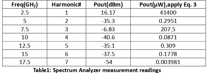
A method is used [2,5] a spectrum analyzer to meas-ure the output harmonics of the amplifier (up to the seventh harmonic in the below example), see Figure 2 for the test setup. The following readings were col-lected from the spectrum analyzer, see Table 1:

Freq(GHZ) Harmonic# Pout(dBm) Pout(µW),apply Eq. 3

2.5 1 16.17 41400

5 2 -35.3 0.2951

7.5 3 -6.83 207.5

10 4 -40.6 0.0871

12.5 5 -35.1 0.309

15 6 -37.5 0.1778

17.5 7 -54 0.003981

Table1: Spectrum Analyzer measurement readings

Using equation one above to calculate the THD, (measured at 2.5 GHz and the output voltage is at 3.6 Vpp):

THD (%) = 100 * sqrt((0.2951E-06 + 207.5E-06 + 0.0871E-06 + 0.309E-06 + 0.1778E-06 + 0.003981E-06)/0.0414) = 7.1%

3. Implementation:

A table is created in Double Precision Floating Point. The following commands make a 256 point sine wave and measure its total harmonic distor-tion when sampled first on the points and then by jumping with a delta of 2.5 points per step using linear interpolation. For frequency-based appli-cations, spectral purity can be more important than absolute error in the table. The M-file is used for calculating total harmonic distortion (THD) for digital sine wave generation with or without inter-polation. This THD algorithm proceeds over an integral number of waves to achieve accurate re-sults[4]. The number of wave cycles used is A.

Since the step size 'delta' is A/B and traversing A waves will hit all points in the table at least one time, which is needed to accurately find the aver-age THD across a full cycle.

The relationship used to calculate THD is:

THD = (ET - EF) / ET, % where ET = total energy, and EF = fundamental energy The energy difference between ET and EF is spu-rious energy. Now the code:

N = 256;

s = sin( 2*pi * (0:(N-1))/N)';

One can put the sine wave designed above into a Simulink model and it can be seen in Figure 4 how it works as a direct lookup and with linear interpo-lation. This model compares the output of the

floating point tables to the sin() function. As expected from the THD calculations, the linear interpolation has a lower error than the direct table lookup in comparison to the sin() function.

Figure 4: Comparison in approximate sine wave accuracy between direct lookup and linear interpolation vs. reference signal

open_system('sldemo_tonegen');

set_param('sldemo_tonegen', 'StopFcn',''); sim('sldemo_tonegen');

figure('Color',[1,1,1]);

subplot(2,1,1), plot(tonegenOut.time, tone-genOut.signals(1).values); grid

title('Difference between direct look-up and reference signal');

subplot(2,1,2), plot(tonegenOut.time, tone-genOut.signals(2).values); grid

title('Difference between interpolated look-up and reference signal');

Figure 5: Difference between direct/interpolated look-up & reference signal

4.8 4.85 4.9 4.95 5 5.05 5.1 5.15 5.2 -0.01

-0.005 0 0.005 0.01

Difference between direct look-up and reference signal

4.8 4.85 4.9 4.95 5 5.05 5.1 5.15 5.2 -5

0 5 10x 10

-5 _{Difference between interpolated look-up and reference signal}

Figure 6: Difference between direct/interpolated look-up & reference signal

Output of the above code is shown in Figure 5 & Figure 6. Taking a Closer Look at Waveform Ac-curacy and Zooming in on the signals between 4.8 and 5.2 seconds of simulation time (for exam-ple), It can be seen a different characteristic due to the different algorithms used:

ax = get(gcf,’Children’); set(ax(2),’xlim’,[4.8, 5.2]) set(ax(1),’xlim’,[4.8, 5.2])

The new table is tested for total harmonic distor-tion in direct lookup mode at 1, 2, and 3 points per step, then with fixed point linear interpolation.

Bits = 24;

is = num2fixpt( s, sfrac(bits), [], ‘Nearest’, ‘on’); thd_direct1 = ssinthd(is, 1, N, 1, ‘direct’)

thd_direct2 = ssinthd(is, 2, N, 2, ‘direct’) thd_direct3 = ssinthd(is, 3, N, 3, ‘direct’)

thd_linterp_2p5 = ssinthd(is, 5/2, 2*N, 5, ‘fixptlinear’)

Results for different tables and methods are

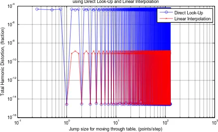
com-pared. Choosing a table step rate of 8.25 points per step (33/4), it was jumped through the double pre-cision and fixed point tables in both direct and li-near modes and compare distortion results in out-put (Figure 7):

thd_double_direct = ssinthd( s, 33/4, 4*N, 33, ‘direct’) thd_sfrac24_direct = ssinthd(is, 33/4, 4*N, 33, ‘direct’)

thd_double_linear = ssinthd( s, 33/4, 4*N, 33, ‘linear’)

thd_sfrac24_linear = ssinthd(is, 33/4, 4*N, 33, ‘fixptlinear’)

10-1 100 101 102 103

10-16

10-14

10-12

10-10

10-8

10-6

10-4

Total Harmonic Distortion for 24-bit 256 point sine wave synthesis table using Direct Look-Up and Linear Interpolation

Jump size for moving through table, (points/step)

T

o

ta

l

H

a

rm

o

n

ic

D

is

to

rt

io

n

,

(f

ra

c

ti

o

n

)

Direct Look-Up Linear Interpolation

Figure 7: Total Harmonic Distortion

4. Test Cases & Observations:

Using Preconfigured Sine Wave Blocks Simulink also includes a sine wave source block with conti-nuous and discrete modes, plus fixed point sin and cosine function blocks that implement the function approximation with a linearly interpolated lookup table that exploits the quarter wave symmetry of sine and cosine.

Now the model is opened by command: open_system('sldemo_tonegen_fixpt');

Survey of Behavior for Direct Lookup and Linear Interpolation The script performs a full frequency

sweep of the fixed point tables will let us more thoroughly understand the behavior of this design. Total harmonic distortion of the 24-bit fractional fixed point table is measured at each step size, moving through it D points at a time, where D is a number from 1 to N/2, incrementing by 0.25 points. N is 256 points in this example, the 1, 2, 2.5, and 3 cases were done above. Frequency is discrete and therefore a function of the sample rate.

error than direct lookup in between points. What wasn't apparent from using common sense was that the error is relatively constant for each of the modes up to the Nyquist frequency.

figure('Color',[1,1,1])

tic, sldemo_sweeptable_thd(24, 256), toc

To take this demonstration further, different table precision and element counts are tried to see the effect of each. One can investigate different im-plementation options for waveform synthesis algo-rithms using automatic code generation available from the Real-Time Workshop and production code generation using Real-Time Workshop(R) Embedded Coder(TM).

bdclose('sldemo_tonegen'); bdclose('sldemo_tonegen_fixpt')

displayEndOfDemoMessage(mfilename)

Embedded Target products offer direct connections to a variety of real-time processors and DSPs, in-cluding connection back to the Simulink diagram while the target is running in real-time.

5. Conclusion:

With the use of non-linear loads on the rise global-ly, isolation for poor quality distribution systems and mitigation of harmonics will become increa-singly important. The limits per IEEE Std 519 are not enforced limits but suggestions on acceptable levels. As a result, THD on certain power systems could be much higher, especially considering the difficulty in attaining harmonic measurements [7].

6. References:

[1].Lundquist, Johan. On Harmonic Distor-tion in Power Systems. Chalmers Univer-sity of Technology: Department of Elec-trical Power Engineering, 2001.

[2].Vic Gosbell. “Harmonic Distortion in the Electrical Supply System,” PQC Tech Note No. 3 (Power Quality Centre), Elliot

Sound Products,

http://sound.westhost.com/lamps/technote 3.pdf

[3].“Harmonics (electrical power).”Wikipedia, The Free Encyclopedia. Wikimedia

Foundation, Inc. 4 April 2011. Web. 5 April 2011.

[4].IEEE Std 519-1992, IEEE Recommended Practices and Requirements for Harmonic Control in Electrical Power Systems, New York, NY: IEEE

[5].Digital Sine-Wave Synthesis Using the DSP56001/DSP56002", by % Andreas Chrysafis, Motorola(R) Inc. 1988

[6].AN 30: Basic Total Harmonic Distortion

(THD) Measurement, CENTELLAX

Speed Innovation