Detecting Quantum Speedup of HHL Algorithm for
Linear Programming Scenarios
Volkan Erol * and Mert Side
Okan University Computer Engineering Department, Tuzla Campus, 34959 Istanbul, Turkey * Correspondence: [email protected]; Tel.: +90-533-3621947
Abstract: Quantum computers are machines that are designed to use quantum mechanics in order to improve upon classical computers by running quantum algorithms. One of the main applications of quantum computing is solving optimization problems. For addressing optimization problems, we can use linear programming. Linear programming is a method to obtain the best possible outcome in a special case of mathematical programming. Application areas of this problem consist of resource allocation, production scheduling, parameter estimation, etc. In our study, we look at quantum speedup ratios of HHL Algorithm for different scenarios of linear programming. In a first scenario we look quantum speedup ratio (S(N)) as a function of phase transition and the ratio (κ) between the greatest and smallest eigenvalues of the matrix in linear equation system. As a second scenario, we investigate the changes in S(N) as a function of κ and s, which is the coefficient for defining the matrix as s-sparse.
Keywords: linear programming; optimization; quantum algorithms; complexity
1. Introduction
Quantum computers are designed to use quantum mechanics to improve speed by running quantum algorithms over classical computers. Entanglement is the theoretical aspect providing the speedup comparing to classical counterparts. Many recent researches have been done in entanglement and its related disciplines like entanglement measures and majorization, etc. [12-20]. One of the main applications of quantum computing is solving optimization problems. Other Application areas of this problem can be listed as resource allocation, production scheduling and parameter estimation, etc.
In our study, we looked at two different scenarios for measuring the quantum speedup in HHL Algorithm. In the first scenario we look at quantum speedup ratio (S(N) defined in the next section) as a function of phase transition ε and the ratio κ between the greatest and smallest eigenvalues of the matrix in linear equation system. As a second scenario, we investigate the changes in S(N) as a function of κ and s, which is the coefficient for defining the matrix as s-sparse.
2. Materials and Methods
Linear optimization (also called linear programming) is a method used to obtain the best result (such as maximum gain or lowest cost) in a mathematical model represented by linear relationships [21-23]. Linear programming is a special case of mathematical programming.
In other words, linear programming is a technique used to optimize a linear objective function, subject to linear equality and linear inequality constraints. The feasible region is a convex polytope, defined as the intersection of the finite half spaces, each defined by a linear inequality. The objective function is a real-valued linear function defined on this polyhedron. A linear programming algorithm finds the smallest (or largest) value on the polyhedron if such a point exists [21-23].
Linear programs are canonical problems that can be expressed as follows:
maximize cTx
subject to Ax ≤ b and x ≥ 0
where x represents the vector of variables (to be determined), c and b are vectors of (known) coefficients, A is a (known) matrix of coefficients, and (.)T is the matrix transpose.
The expression to be maximized or minimized is called an objective function (in this case cTx). Ax ≤ b and x ≥ 0 inequalities are constraints that specify a convex polytope on which the
objective function is optimized. In this context, two vectors are comparable when they have the same dimensions. If each leading input is less than or equal to the corresponding input of the second, we can say that the first vector is less than or equal to the second vector [21-23].
Linear programming can be applied to various fields of study. It is widely used in business and economics, and is also used for some engineering problems. Industries using linear programming models include transportation, energy, telecommunications and manufacturing. It has proven useful in modeling various types of problems in planning, routing, scheduling, assignment and design.
A fundamental task in mathematics, engineering and many areas of science is solving systems of linear equations. This problem is defined as follows: We are given an N × N matrix A, and a vector b ∈ RN, and are asked to output x such that Ax = b. This problem can
be solved in time polynomial in N by linear algebra methods such as Gaussian elimination. These works are reviewed by Montanaro [11].
The quantum algorithm of Harrow, Hassidim and Lloyd [1] (HHL) for solving systems of linear equations sidesteps this issue by “solving” the equations in a peculiarly quantum sense:
outputs a state approximately proportional to x =
iN=1xi i . This is an N-dimensional quantum state which can be stored in O(logN) qubits.This algorithm gives a solution of linear equations of type Ax = B [1], where A is a s-sparse matrix. This algorithm has time complexity:
Õ(log(N)κ2s2/ε) (1)
where κ is the proportion of the greatest eigenvalue to the smallest eigenvalue in the matrix and ε is the phase estimation error bound constant [1, 3].
If non-zero element count d in rows and κ are small, this is an exponential improvement on standard classical algorithms. Indeed, one can even show that achieving a similar runtime classically would imply that classical computers could efficiently simulate any polynomial-time quantum computation [1].
Of course, rather than giving as output the entirety of x, the algorithm produces an N-dimensional quantum state x ; to output the solution x itself would then involve making many measurements to completely characterise the state, requiring time of order N in general. However, we may not be interested in the entirety of the solution, but rather in some global property of it. Such properties can be determined by performing measurements on x . For example, the HHL algorithm allows one to efficiently determine whether two sets of linear equations have the same solution [3], as well as many other simple global properties [4].
The HHL algorithm is likely to find applications in settings where the matrix A and the vector b are generated algorithmically, rather than being written down explicitly. One such setting is the finite element method (FEM) in engineering. Recent work by Clader, Jacobs and Sprouse has shown that the HHL algorithm, when combined with a preconditioner, can be used to solve an electromagnetic scattering problem via the FEM [4]. The same algorithm, or closely related ideas, can also be applied to problems beyond linear equations themselves. These include solving large systems of differential equations [5, 6], data fitting [7] and various tasks in machine learning [8]. It should be stressed that in all these cases the quantum algorithm “solves” these problems in the same sense as the HHL algorithm solves them: it starts with a quantum state and produces a quantum state as output. Whether this is a reasonable definition of “solution” depends on the application, and again may depend on whether the input is produced algorithmically or is provided explicitly as arbitrary data [9].
The simplex method is a method for solving problems in linear programming. This method, invented by George Dantzig in 1947, tests adjacent vertices of the feasible set (which is a polytope) in sequence so that at each new vertex the objective function improves or is unchanged [10]. The simplex method is very efficient in practice, generally taking 2m to 3m
3. Results
For defining the quantum speedup Ronnow et. al. proposed a classical to quantum scaling ratio [24]:
S(N) = C(N)/Q(N) (2) where C(N) is the time used by a classical device to solve a problem of size N and Q(N) is the time used on a quantum device. S(N) > 1 means that there is a quantum speed up in the setup.
Worst-case time complexity of Simplex is O(nm) where n is the number of variables and m is the inequality constraints [2]. Average time complexity of Simplex is O((n+m)*n). For our example problem setup in the definition of C(N) we use the previously mentioned average time complexity, therefore, C(N) = N2+4N.
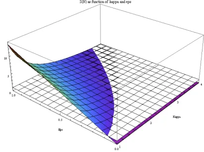
In the first setup we look at S(N) as a function of κ and ε. In Figure 1, it can be viewed that there is quantum speedup in many cases (region of the 3D plot which is above the plane z=1). Maximum quantum speedup ratio is around 13. For the values ε > ~0.85 we cannot view quantum speedup. Similarly, for κ > 3.6~, we cannot view quantum speedup.
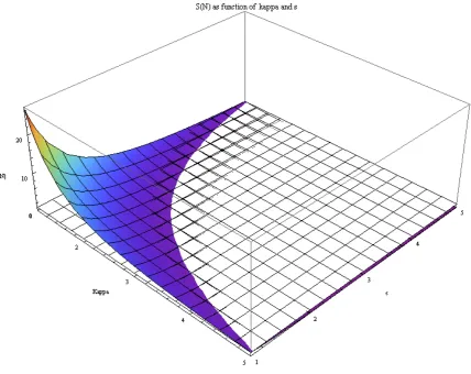
In the second scenario, in Figure 2, we visualize the changes in S(N) as a function of
κ and s. The maximum quantum speedup ratio achieved is ~30 and the regions above the plane z=1 show the parts of the 3D plot where quantum speedup occurs.
Figure 2. Quantum speedup ratio-S(N) as a function of κ and s (coefficient of s-sparse matrix)
4. Discussion
References
1. A. W. Harrow, A. Hassidim, S. Lloyd, Phys. Rev. Lett. vol. 15, no. 103, pp. 150502 (2009).
2. A. H. G. Rinnoy Kan, J. Telgen, The complexity of linear programming, Statistica Neerlandica, nr. 2 (1981).
3. A. Ambainis. Variable time amplitude amplification and a faster quantum algorithm for solving systems of linear equations. In Proc. 29th Annual Symp. Theoretical Aspects of Computer Science, pages 636–647 (2012).
4. B. Clader, B. Jacobs, and C. Sprouse. Preconditioned quantum linear system algorithm. Phys. Rev. Lett., 110:250504, (2013).
5. S. Leyton and T. Osborne. A quantum algorithm to solve nonlinear differential equations, arXiv:0812.4423 (2008).
6. D. Berry. High-order quantum algorithm for solving linear differential equations. J. Phys. A: Math. Gen., 47 105301, (2014).
7. N. Wiebe, D. Braun, and S. Lloyd. Quantum algorithm for data fitting. Phys. Rev. Lett., 109 050505, (2012).
8. S. Lloyd, M. Mohseni, and P. Rebentrost. Quantum algorithms for supervised and unsupervised machine learning, arXiv:1307.0411, (2013).
9. S. Aaronson. Quantum machine learning algorithms: Read the fine print. Nature Physics, 11 p.291– 293, (2015).
10. G. B. Dantzig, Linear Programming and Extensions. Princeton University Press (Princeton, NJ) (1963).
11. A. Montanaro, Quantum algorithms: an overview, npj Quantum Information vol. 2, 15023 (2016).
12. V. Erol, F. Ozaydin, A. A. Altintas, Analysis of entanglement measures and locc maximized quantum fisher information of general two qubit systems, Sci. Rep. 4, 5422 (2014).
13. F. Ozaydin, A. A. Altintas, C. Yesilyurt, S. Bugu, V. Erol, Quantum Fisher Information of Bipartitions of W States, Acta Physica Polonica A 127, 1233-1235 (2015).
14. V. Erol, S. Bugu, F. Ozaydin, A. A. Altintas, An analysis of concurrence entanglement measure and quantum fisher information of quantum communication networks of two-qubits, Proceedings of IEEE 22nd Signal Processing and Communications Applications Conference (SIU2014), pp. 317-320, (2014).
15. V. Erol, A comparative study of concurrence and negativity of general three-level quantum systems of two particles, AIP Conf. Proc. 1653 (020037), (2015).
17. V. Erol, Detecting Violation of Bell Inequalities using LOCC Maximized Quantum Fisher Information and Entanglement Measures, Preprints 2017, 2017030223 (doi: 10.20944/preprints201703.0223.v1) (2017).
18. V. Erol, Analysis of Negativity and Relative Entropy of Entanglement Measures for Two Qutrit Quantum Communication Systems, Preprints 2017, 2017030217 (doi: 10.20944/preprints201703.0217.v1) (2017).
19. V. Erol, The relation between majorization theory and quantum information from entanglement monotones perspective, AIP Conf. Proc. 1727 (020007), (2016).
20. V. Erol, A Proposal for Quantum Fisher Information Optimization and its Relation with Entanglement Measures, PhD Thesis, Okan University, Institute of Science, (2015).
21. G. Sierksma, Linear and Integer Programming: Theory and Practice, Second Edition. CRC Press. p. 1. (2001).
22. Alexander Schrijver, Theory of Linear and Integer Programming. John Wiley & Sons. pp. 221– 222. (1998).
23. G. B. Dantzig, Reminiscences about the origins of linear programming, Operations Research Letter. 1 (2): 43–48, (1982).
24. T. F. Ronnow et al, Defining and detecting quantum speedup, Science 345, 420 (2014).