Undirected Graphs: Is the Shift- Enabled Condition Trivial or Necessary?

Undirected

Graphs:

I

s

the

Shift-

E

nabled

Condition

Trivial

or

Necessary?

LiyanChen1,† ,SamuelCheng1,3,†*,KanghangHe4,LinaStankovic4andVladimirStankovic4 1 _{College of Electronic and Information Engineering, Tongji University; [email protected]}

2 _{Key Laboratory of Oceanographic Big Data Mining & Application of Zhejiang Province, Zhejiang Ocean}

University

3 _{the School of Electrical and Computer Engineering, University of Oklahoma} 4 _{the Department of Electronic and Electrical Engineering, University of Strathclye}

* Correspondence: [email protected] † 4800 Caoan Road, Shanghai, P.R. China

1

2

3

4

5

6

7

8

9

10

Abstract: Ithasrecentlybeenshownthat,contrarytothewidebeliefthatashift-enabledcondition

(necessaryforanyshift-invariantfiltertoberepresentablebyagraphshiftmatrix)canbeignored

becauseanynon-shift-enabledmatrixcanbeconvertedtoashift-enabledmatrix,suchaconversion

ingeneralmaynotholdforadirectedgraphwithnon-symmetricshiftmatrix.Thispaperextends

thispriorwork,focusingonundirectedgraphswheretheshiftmatrixisgenerallysymmetric.We

showthatwhile,inthiscase,theshiftmatrixcanbeconvertedtosatisfytheoriginalshift-enabled

condition,theconvertedmatrixisnotassociatedwiththeoriginalgraph,thatis,itdoesnotcapture

anymorethestructureofthegraphsignal.Weshowviaacounterexample,thatanon-shift-enabled

matrixcannotbeconvertedtoashift-enabledoneandstillmaintainthetopologicalstructureofthe

underlyinggraph,whichisnecessarytofacilitatelocalizedsignalprocessing.

Keywords: graphsignalprocessing;shift-enabledgraphs;shift-invariantfilter;undirectedgraph

11

1. Introduction

12

Graph signal processing (GSP) extends classical digital signal processing (DSP) to signals on

13

graphs, and provides a prospective solution to numerous real-world problems that involve signals

14

defined on topologically complicated domains, such as social networks, point clouds, biological

15

networks, environmental and condition monitoring sensor networks [1]. However, there are several

16

challenges in extending classical DSP to signals on graphs, particularly related to the design and

17

application of graph filters.

18

In classical, one-dimensional DSP, any linear, time-invariant, or shift-invariant, filter that

19

commutes with time shift operator z−1 can be represented as a polynomial of z−1 leading to

20

Z-transform of the filter. Conversely, if a linear filter can be represented as a polynomial ofz−1,

21

the filter is linear and shift-invariant. Unfortunately, this concept does not simply generalize to

22

GSP, partly because the definition of a “shift" for a graph is not obvious [2]. Commonly, in the GSP

23

literature, a graph is uniquely described by a “shift” matrix or a “shift" operator1,S[3–5], which has

24

been extensively used for time/vertex-domain filter design (see [1], [2] and references therein for

25

frequency-domain and time/vertex-domain filtering). For example, adjacency matrix, for general

26

graphs, and Laplacian matrix, for undirected graphs, are some popular choices for the shift matrix.

27

In order to make graph filtering feasible, even for very large graphs, it is necessary to perform the

28

filtering operation locally. For example, consider a sensor network represented by a graph, where the

29

edges and edge weights of the graph depend on the distance between the sensors. In this case, efficient

30

1 _{The term “shift” comes from the analogy withz}−1_{operator inZ−transform of classical DSP.}

filtering boils down to merely mixing the signals acquired by a sensor with those of the nearest sensors.

31

Otherwise, if the filter output at any graph vertex is a linear combination of inputs atallvertices,

32

filtering will be practically infeasible for “big data" graphs [5]. Therefore, in practice, we expect that a

33

node can only impose direct influence to an adjacent node through the shift operator. For practical

34

design purposes, it is advantageous to be able to decompose filters in a form of polynomial of such a

35

shift matrix. The importance of this polynomial representation has been reiterated in a recent survey

36

paper (see Section II.F of [1]).

37

Although a nice, but loose, analogy betweenSandz−1can be established [1], unlike classical

38

DSP, if a graph filter is shift-invariant (the shift matrix commutes with the target filter), this does not

39

automatically imply that a polynomial representation of the filter exists [6]. Ref. [3] argues that, for

40

any shift matrixS, there exists a converted shift matrix ˜Ssuch that graph filterHis a polynomial in

41

˜

S. However, it is not sufficient just to haveHto be represented as a polynomial of any arbitrary ˜S.

42

One should also ensure thatS indeed describes the same graph as S˜ (see details in Definition2), that is, the

43

converted graph shift should keep the same topological structure as the original one.

44

1.1. Contribution

45

It was shown in [3] that any filter commuting with shift matrix S can be represented as a

46

polynomial in S provided that the characteristic and minimal polynomial of the shift matrix are

47

equal (in the rest of this paper, as in [7], we will refer to this condition asshift-enabled condition, see also

48

Definition1). However, in [3], this condition was immediately disregarded, surmising that one may

49

convert any shift matrix that does not satisfy the shift-enabled condition into one that does. Based on

50

this conclusion, most researchers currently assume that the shift-enabled condition simply holds or

51

ignore the condition completely. However, it was proved in [7], through a counterexample, that such a

52

conversion may not hold for a directed graph with asymmetric shift matrix.

53

In this paper, we focus on undirected graphs, which have wider applications [2], and illustrate

54

with examples that when the symmetric shift matrix of an undirected graph is non-shift-enabled, the

55

conversion suggested in [3] could lead to a very different graph that does not necessarily capture the

56

structure of the original graph signal. Namely, though the conversion would provide a shift-enabled

57

graph that facilitates polynomial representation of the shift-invariant filters, the newly designed graph

58

might no longer capture the structure of the graph signal it was originally designed to model2, and

59

does not facilitate performing filtering locally.

60

Referring to our wireless sensor network example in the introduction, in the original graph the

61

output of the filtering at each vertex only involves inputs of the vertex’s immediate neighborhoods.

62

However, in the converted graph, sensors that are far apart might be strongly connected, that is, each

63

output at a vertex could be a linear combination of inputs at almost all vertices, thus filtering in such

64

converted graph will be computationally unaffordable for “big data” graphs in practice which further

65

emphasizes the importance of the shift-enabled condition [7].

66

The outline of the paper is as follows. Section2describes the basic concepts and key properties of

67

a shift-enabled graph. Section3provides counterexamples to prove that the shift-enabled condition is

68

essential for the symmetric graph. Section4concludes the paper.

69

2. Basic Concepts and Properties of Shift-enabled Graphs

70

In this section, we briefly review the concepts of shift-enabled graphs and their properties relevant

71

to this paper. For more details, see [2–5].

72

LetG= (V,A)be a graph, whereV={v0,v1,· · ·,vn−1}is a set of vertices and A∈Cn×nis the

73

adjacency matrix of the graph. Letx= (x0,x1,· · ·,xn−1)Tbe agraph signal, where each samplexi∈x

74

corresponds to a vertexvi∈V.

75

In particular, ifGis a directed circular graph, then the corresponding adjacency matrix is given by:

76

A= 



0 0··· 0 1 1 0··· 0 0

..

. ... ... ...

0 0··· 1 0 

. Then Ax= (xn−1,x0,· · ·,xn−2)T, that is, multiplication byAshifts each signal

77

sample to the next vertex. Thus,Ais often called shift operator or shift matrix, which is similar to

78

time shift operatorz−1in DSP. In practice, adjacency matrix can be replaced by other matrices which

79

reflect the structure of the graph, such as the Laplacian matrix and the normalized Laplacian matrix

80

for undirected graphs, and the probability transition matrix. Here, we useSto denote the general shift

81

matrix, whether it isA, (normalized) Laplacian matrix, or the probability transition matrix.

82

In classical 1-D DSP, a shift-invariant filterFhas aZ-transform (polynomial representation in

z−1), that is

F(z−1) =

+∞

∑

fkz−k,

where fkis polynomial coefficient. Moreover, from the shift-invariance property, it follows that the

83

filtered output of a shifted input is equal to the shifted filtered output of the original input. In other

84

words, the shift operation and the filter commute. That is,Fz−1=z−1F, which directly follows from

85

the above polynomial representation (see, e.g., [6]).

86

Extending this concept to GSP, we also define a shift-invariant filterHas the one that commutes

87

with the shift matrix, i.e.,HS=SH. However, unlike in the classical DSP case, a shift-invariant filter

88

does not necessarily have a polynomial representation in terms of the shift operatorS. Yet,Hcan be

89

represented as a polynomial inSif the shift matrixSsatisfies the following condition.

90

Definition 1(Shift-enabled graph [7]). A graphGis shift-enabled if its corresponding shift matrix S satisfies

91

pS(λ) =mS(λ), where pS(λ)and mS(λ)are the minimum polynomial and the characteristic polynomials of

92

S, respectively. We also say that S is shift-enabled when the above condition is satisfied. Otherwise, S and the

93

corresponding graph, are non-shift-enabled.

94

For shift-enabled graphs, the following theorem is the basis of linear, shift-invariant filter design.

95

Theorem 1. The shift matrix S is shift-enabled if and only if every matrix H commuting with S is a polynomial

96

in S[3].

97

Note that this theorem implies that as long as the shift matrixSdoes not satisfy the shift-enabled

98

condition (i.e.,mS(λ)6=pS(λ)), there will always be some shift-invariant filters (and thus some filters)

99

that cannot be represented as a polynomial ofS. Ref [3] de-emphasized the shift-enabled condition by

100

suggesting that we may work around it with the following theorem.

101

Theorem 2(Theorem 2 in [3]). For any shift matrix S, there exists a converted matrixS and matrix polynomial˜

102

r(·), such that S=r(S˜)and m_S˜(λ) =p_S˜(λ).

103

While the above theorem is correct, it does not take into account that the target filterHmay not

104

be shift-invariant with respect to the converted shift matrix. In particular, for a directed graph, in

105

general,Sis not symmetric, and thus not jointly diagonalized withH. Consequently, one can show

106

that generally there exists no converted shift-enabled ˜Sthat can maintain shift-invariance with the

107

target filter when the graph is directed andSis asymmetric [7].

108

However, the conversion method suggested in [3] does hold for undirected graphs when H

109

can be jointly diagonalized withS. Yet, as we will show in the following, the converted ˜Smay not

110

describe the same graph as the originalS. This makes the whole conversion process moot. Hence, the

shift-enabled condition is important regardless of whether the graph is directed or not (i.e., the shift

112

matrix is asymmetric or not).

113

3. The Necessity of Shift-enabled Condition for Undirected Graphs

114

Before giving a concrete example, let us first review the conversion process described in [3]. As

115

mentioned earlier, even though the conversion process does not hold for arbitrary shift matrices, it can

116

be applied to symmetric shift matrices.

117

According to LemmaA2in Appendix A, two symmetric and commuting matricesSandHare

118

simultaneously diagonalizable. Thus, there exists an invertible matrixTsuch thatS=TΛST−1and

119

H= TΛHT−1, whereΛSandΛHare composed of the eigenvalues ofSandH, respectively. Then,

120

a new matrixΛperturb with distinct diagonal elements can be generated by slightly perturbing the

121

values ofΛS. The new shift matrix is calculated as ˜S =TΛperturbT−1. According to LemmaA1and

122

LemmaA2, the restructured shift matrix ˜Ssatisfies p_S˜(λ) = m_S˜(λ)andHS˜ = SH˜ . Hence, from

123

Theorem1,His a polynomial in ˜S.

124

However, it is not sufficient to haveHrepresented as a polynomial of any arbitrary ˜S. A natural

125

and basic constraint is that the converted ˜Sshould facilitate “local processing”, that is, it should

126

describe topologically the same graph, which is essential in virtually all GSP applications, such as filter

127

design [8], sampling [9], denoising [10], and classification [11], otherwise, the conversion is meaningless.

128

To ensure that the converted graph facilitates “local processing”, that is, an implementation of an

129

L-th order polynomial filter requiresLdata exchanges between neighbouring nodes [6], we introduce

130

Definition2. In fact, the definition of a matrix describing a graph (see details in Definition2) is not new

131

in spectral graph theory. In particular, the matrix of “loose description” is widely used in the context of

132

inverse eigenvalue problem and zero-forcing problem [12,13]. We introduce “strict description” since

133

we would like to accommodate graphs with self-loops. In a nutshell, two shift matrices describe the

134

same graph if the conversion from one to another preserves the graph topological structure, implying

135

that filtering under the converted graph can be performed locally. The precise definition is specified as

136

follows.

137

Definition 2([12–14]). Shift matrices S andS strictly describe the same graph if 1) S˜ i,j 6=0if and only if

138

˜

Si,j 6=0for any i and j, and 2)S is symmetric if and only if S is symmetric. And we will say S and˜ S loosely˜

139

describe the same graph if the first condition is relaxed to 1’) Si,j6=0if and only ifS˜i,j 6=0only for i6=j. That

140

is, we allow some i where only Si,iorS˜i,iequal to0.

141

Given this additional constraint that ˜SandSshould describe the same graph structure, we can

142

show that it is impossible to guarantee the following three conditions to be satisfied simultaneously:

143

• S˜is shift-enabled (i.e.,pS˜(λ) =mS˜(λ)).

144

• His shift-invariant on ˜S(i.e.,HS˜=SH˜ ).

145

• S˜andSstrictly or loosely describe the same graph.

146

3.1. A counter-example thatS can loosely but not strictly describe the original graph˜

147

Let us start with a non-shift-enabled graph as shown in Figure.1(a). The shift matrix3of the

148

undirected graph isS=

0 1 1 1 1 1 0 0 0 0 1 0 0 0 0 1 0 0 0 0 1 0 0 0 0 !

. It is clear that pS(λ) =λ3(λ−2) (λ+2)6=λ(λ−2) (λ+2) =

149

mS(λ)and henceSis non-shift-enabled. Since shift-enabled condition is not just sufficient but also

150

necessary [7], there must exist a shift-invariant filter not representable as a polynomial ofS. Indeed,

151

1

5 2

4

3

(a)

1

5 2

4

3

(b) (c)

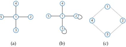
Figure 1.Graph topology used in the examples. (a) Original graph with shift matrixS. (b) Converted shift matrix ˜Swhich loosely describes the same graph asS. (c) Cycle graph with shift matrixS0.

one example for such a filter isH=





0 0 0 0 0 0 1 −1 0 0 0−1 1 0 0 0 0 0 0 0 0 0 0 0 0



. It can be readily verified thatHS=0=SHand

152

thus the filter is shift-invariant, and it is impossible to find polynomial representation ofHin terms of

153

S. Note thatSn

2,3=Sn2,44for alln∈N. Thus for any polynomialh(S), we must haveh(S)2,3=h(S)2,4.

154

But sinceH2,3=−16=0=H2,4,H6=h(S)for any polynomial functionh(·).

155

3.1.1. Extension ofHto a Class of Filters

156

Note that we can extendH to the following class of filters that all cannot be represented as

polynomials ofS:

H={αH+q(S)|α∈R,q(S)is a polynomial ofS}. (1)

Since apparentlyq(S)S=Sq(S)for any polynomialq(S)andHS=SHas discussed above, any

157

filterαH+q(S)∈Hcommutes withSas well. Thus any filter inHis shift-invariant. However, since

158

His not representable as a polynomial ofS, as discussed above, so doesαH+q(S).

159

From the examples presented above, we note that when the shift-enabled condition is violated,

160

we may find an infinite number of shift-invariant filters that are not representable as polynomials ofS.

161

3.1.2. Shift-enabled ˜SThat Strictly Describes the Original Graph Does Not Exist

162

First, let us restrict the converted shift matrix ˜Sto strictly describe the same graph asS. Thus ˜S

could be written as

˜

S= 

  

0 S˜1,2S˜1,3S˜1,4 S˜1,5 ˜

S1,2 0 0 0 0 ˜

S1,3 0 0 0 0 ˜

S1,4 0 0 0 0 ˜

S1,5 0 0 0 0 

  

(2)

with non-zeros ˜S1,2, ˜S1,3, ˜S1,4, and ˜S1,5. We can readily verify that the characteristic polynomial is

163

pS˜(λ) =λ3(λ2−S˜212−S˜132 −S˜214−S˜215)and 0 is the triple eigenvalue of ˜S. According to LemmaA1, a

164

shift-enabled real symmetric shift matrix has to have unique eigenvalues and thus ˜Sis not shift-enabled.

165

Therefore, all graphs which have the same structure as Figure1(a)are non-shift-enabled.

166

3.1.3. Shift-enabled ˜SThat Loosely Describes the Original Graph Exists

167

Next, let us relax ˜Sso that it may just loosely describe the original graph. In other words, we

allow the diagonal elements to be non-zero which maintains most of the topological structure of the original graph. In applications where diffusion or state transition matrices are treated as shift matrices,

4 _{Note thatS}k

the diagonal elements can be interpreted as the returning probabilities of the current state to itself. Thus, the converted shift matrix ˜Scan be written as

˜

S= 

   ˜

S1,1 S˜1,2S˜1,3S˜1,4S˜1,5 ˜

S_1,2 S˜2,2 0 0 0 ˜

S_1,3 0 S˜3,3 0 0 ˜

S1,4 0 0 S˜4,4 0 ˜

S1,5 0 0 0 S˜5,5 

 

. (3)

Many solutions that satisfy shift-enabled and shift-invariant conditions can be found. For instance,

168

˜

S=

0 1 1 1 1 1 1 0 0 0 1 0 1 0 0 1 0 0 0 0 1 0 0 0 0 !

is one such solution, where the original graph structure is only slightly modified as

169

shown in Figure1(b). One can verify that the eigenvalues(−1.8136, 0, 0.4707, 1, 2.3429)of ˜Sare distinct

170

and thus ˜Sis shift-enabled. Moreover, one can also readily verify thatHS˜=SH˜ . By Theorem 1, the

171

above two conditions ensure thatHis a polynomial in ˜S.

172

Remark 1. Note that the example from the previous section can be extended to a star graph with more than five vertices. In this case, the shift matrix of a star graph with N vertices is SN =



 0 1··· 1 1 0··· 0 .. . ... ... 1 0··· 0



. Consider a

filter HN = 

  

0 0 0 0 ··· 0 0 1 −1 0··· 0 0−1 1 0 ··· 0 0 0 0 0 ··· 0 ..

. ... ... ... ... ... 0 0 0 0 ··· 0



  

, and based on Equation2shift operator that strictly describing the original

graph satisfiesS˜N(strict)=



   

0 S˜1,2S˜1,3 ··· S˜1,N

˜

S1,2 0 0 ··· 0 ˜

S1,3 0 0 ··· 0 ..

. ... ... ... ... ˜

S_1,N 0 0 ··· 0 

   

. Repeating the similar argument as before, we can readily

verify that the following five conclusions still hold simultaneously: (i) SNis not shift-enabled for pSN(λ) =

λN−2(λ2−(N−1)). (ii) HN is shift-invariant, i.e., HNSN = 0 = SNHN. (iii) HN 6= h(SN)for any polynomial function hN(·). (iv) HNcan be extended to the following class of filters that none can be represented as polynomials of SN:

HN={αHN+q(SN)|α∈R,q(SN)is a polynomial of SN}. (v) Shift-enabledS˜N(strict)that strictly describes the original graph does not exist. 173

3.2. A Counter Example When the Converted Shift Matrix Can Neither Strictly Nor Loosely Describe the

174

Original Graph

175

Note that there are situations where no shift-enabled ˜S exists even after we relax the graph

176

structure constraint as in the earlier example. Consider shift matrixS0 =

0 1 0 1 1 0 1 0 0 1 0 1 1 0 1 0

as shown in

177

Figure1(c).

178

It can easily be seen that the eigenvalues of S0, (0, 0, 2,−2), are not unique. Thus S0 is

179

non-shift-enabled according to LemmaA1. So we do expect that there exists shift-invariant filter

180

not representable byS0. Indeed, we can easily show that filterH0 =

0 0 −1 1 0 −1 1 0 −1 1 0 0 1 0 0 −1

!

is such a filter.

181

First, note thatH0S0 = S0H0 and thus H0 is shift-invariant underS0. Furthermore, note that

182

(S0)n_1,2 = (S0)n_1,4 for alln ∈ _N, and soh(S0)1,2 = h(S0)1,4for any polynomialh(S0). But sinceH_1,20 =

183

06=1=H_1,40 ,H0 =6 h(S0)for any polynomial functionh(·).

184

Let us prove that it is impossible to find a converted shift matrix ˜S0_{which is shift-enabled and}

185

commutes withH0by only changing the weights of nonzero and diagonal elements.

Consider a general symmetric matrix

˜

S0 ₌ 

  ˜

S01,1 S˜01,2 0 S˜01,4 ˜

S0

1,2 S˜02,2S˜02,3 0 0 S˜0

2,3S˜03,3S˜03,4 ˜

S0

1,4 0 S˜03,4S˜04,4 



 (4)

which has arbitrary weights on nonzero and diagonal elements. That is, ˜S0loosely describes the same

187

graph asS0.

188

H0=h(S˜0_{)clearly implies thatH}0_{commutes with ˜S}0_{, namely,H}0_S˜0_=S˜0_H0_{is a necessary condition} forH0 =h(S˜0_{). It follows fromH}0_S˜0_=S˜0_H0_{that ˜S}0

1,1 =S˜02,2=S˜03,3=S˜04,4and ˜S01,2=S˜01,4=S˜02,3=

˜

S03,4, i.e.,

˜

S0 ₌ 

  ˜ S0

1,1S˜01,2 0 S˜01,2 ˜

S0

1,2S˜01,1 S˜01,2 0 0 S˜0

1,2 S˜01,1S˜01,2 ˜

S0

1,2 0 S˜01,2S˜01,1 



. (5)

Following Cayley-Hamilton Theorem [15], if H0 is a polynomial in ˜S0_{, then H}0 _{= h(S˜}0_{) =}

189

h0I+h1S˜0+h2S˜0 2

+h3S˜0 3

, whereIas the identity matrix. In fact, it is easy to prove that(S˜0₎k

1,2= (S˜0)1,4k ,

190

fork=0, 1, 2, 3. Hence,h(S˜0)1,2 =h(S˜0)1,4which contradicts withH1,20 6= H1,40 . Thus, for this example,

191

the filterH0cannot be represented as a polynomial in the converted shift matrix ˜S0_{which even just}

192

loosely describes the original graph.

193

Remark 2. Just as in Remark 1, the above example can be extended to cycle graphs with more vertices.

194

In this case, the shift matrix of cycle graph with N vertices is S0_N = 

 

0 1 0··· 0 1 1 0 1··· 0 0 0 1 0··· 0 0 ..

.... ... ... ... ... 1 0 0··· 1 0





. Consider the filter

195

H0_N= 

  

0 0 ··· 0 −1 1 0 0 ··· −1 1 0 0 0 ··· 1 0 0 ..

. ... ... ... ... −1 1··· 0 0 0 1 0 ··· 0 0 −1



  

, and similar to Equation4, the shift operators loosely describing the original graph

196

should satisfyS˜0N(loose) =

      ˜ S0

1,1 S˜01,2 0 ··· S˜01,N

˜ S0

1,2 S˜02,2S˜02,3 ··· 0 0 S˜0

2,3S˜03,3 ··· 0 ..

. ... ... ... ... ˜

S0

1,N 0 0 ··· S˜0N,N

     

. With the similar argument as before, one can show

197

thatS˜0N(shi f t−invariant)=

      ˜ S0

1,1 S˜01,2 0 ··· S˜01,2 ˜

S0

1,2 S˜01,1S˜01,2 ··· 0 0 S˜01,2S˜01,1 ··· 0 ..

. ... ... ... ... ˜

S0

1,2 0 0 ··· S˜01,1      

. Consequently, one can readily verify the following four

198

conclusions in Section3.2are still valid: (i) S0_Nis not shift-enabled, since it has repeated eigenvalues, that

199

is,λk = 2cos(2πk/N)for k = 0, 1, 2,· · ·,N−1. (ii) H0Nis shift-invariant, i.e., H0NS0N = S0NHN0 . (iii)

200

H0_N6=h(S0_N)for any polynomial function hN(·). (iv) The shift matrix that loosely describes the original graph

201

and commutes with H_N0 must have the form ofS˜0

N(shi f t−invariant), and such a shift-enabled matrix does not 202

exist.

203

4. Conclusions

204

For a non-shift-enabled graph, even if we can easily “transform" the symmetric shift matrixS

205

into one that satisfies the shift-enabled condition, the new ˜Smay be irrelevant since it describes a

206

very different graph fromS. That is, the operator ˜Son a graph signal may involve mixing inputs far

207

beyond its neighborhood and become impractical for huge graphs. Combined with the necessity of

208

the shift-enabled condition for directed graph [7], we demonstrated in this paper that the shift-enabled

209

condition is essential for any graph structure. A good future direction is to explore a shift that

“approximately" describes the original graph as the conversion is quite different. In particular, if it is

211

already known that one such shift does not exist, one possible direction to explore shift “approximately"

212

describe the original graph instead (some non-zero off diagonal element may not correspond to an

213

actual edge). But we will leave this to future study.

214

Note that even though we consider the adjacency matrix as the shift matrix in our examples, the

215

conclusion applies to other shift matrices. In particular, one can readily verify that the conclusion still

216

holds if we use the Laplacian matrix as the shift matrix in the example in Section3.2.

217

Author Contributions: writing–original draft preparation, Liyan Chen and Samuel Cheng; writing–review and

218

editing, Lina Stankovic and Vladimir Stankovic; methodology, Kanghang He.

219

Funding:This research was funded by the European Union‘s Horizon 2020 research and innovation programme

220

under the Marie Sklodowska-Curie grant agreement number 734331, the Fundamental Research Funds for

221

the Central Universities number 0800219369 and National Key Research and Development Project number

222

2017YFE0119300.

223

Acknowledgments:The authors thank B. Zhao for helpful discussions.

224

Appendix A

225

It is easily determined whether a graph is shift-enabled by the following lemmas.

226

Lemma A1. If shift matrix S is a real symmetric matrix, then S is shift-enabled, if and only if all eigenvalues of

227

S are distinct [1].

228

LemmaA1indicates that an undirected graph is shift-enabled if and only if its eigenvalues are all

229

distinct.

230

As both shift matrixSand filter matrixHare symmetric, we can obtain the following lemma.

231

Lemma A2. If shift matrix S and filter matrix H are diagonalizable (this condition always holds for symmetric

232

matrix) then S and H are simultaneously diagonalizable (by an invertible matrix) if and only if HS=SH(see

233

Theorem 1.3.12 in [16]).

234

References

235

1. Ortega, A.; Frossard, P.; Kovaˇcevi´c, J.; Moura, J.M.; Vandergheynst, P. Graph signal processing: Overview,

236

challenges, and applications. Proceedings of the IEEE2018,106, 808–828.

237

2. Shuman, D.I.; Narang, S.K.; Frossard, P.; Ortega, A.; Vandergheynst, P. The emerging field of signal

238

processing on graphs: Extending high-dimensional data analysis to networks and other irregular domains.

239

IEEE Signal Proc. Magazine2013,30, 83–98.

240

3. Sandryhaila, A.; Moura, J.M. Discrete signal processing on graphs. IEEE Trans. Signal Processing2013,

241

61, 1644–1656.

242

4. Sandryhaila, A.; Moura, J.M. Discrete Signal Processing on Graphs: Frequency Analysis. IEEE Trans. Signal

243

Processing2014,62, 3042–3054.

244

5. Sandryhaila, A.; Moura, J.M. Big data analysis with signal processing on graphs: Representation and

245

processing of massive data sets with irregular structure.IEEE Signal Processing Magazine2014,31, 80–90.

246

6. Teke, O.; Vaidyanathan, P. Linear systems on graphs. 2016 IEEE Global Conference on Signal and

247

Information Processing (GlobalSIP). IEEE, 2016, pp. 385–389.

248

7. Chen, L.; Cheng, S.; Stankovic, V.; Stankovic, L. Shift-enabled graphs: Graphs where shift-invariant filters

249

are representable as polynomials of shift operations.IEEE Signal Processing Letters2018,25, 1305–1309.

250

8. Hammond, D.K.; Vandergheynst, P.; Gribonval, R. Wavelets on graphs via spectral graph theory. Applied

251

and Computational Harmonic Analysis2011,30, 129–150.

252

9. Gadde, A.; Anis, A.; Ortega, A. Active semi-supervised learning using sampling theory for graph signals.

253

Proc. 20th ACM SIGKDD Intl. Conf. Knowledge Discovery & Data Mining, 2014, pp. 492–501.

254

10. Yang, C.; Cheung, G.; Stankovic, V. Estimating heart rate and rhythm via 3D motion tracking in depth

255

video.IEEE Transactions on Multimedia2017,19, 1625–1636.

11. He, K.; Stankovic, L.; Liao, J.; Stankovic, V. Non-Intrusive Load Disaggregation Using Graph Signal

257

Processing. IEEE Transactions on Smart Grid2018,9, 1739–1747.

258

12. Hogben, L. Spectral graph theory and the inverse eigenvalue problem of a graph. Electronic Journal of

259

Linear Algebra2005,14, 3.

260

13. Trefois, M.; Delvenne, J.C. Zero forcing number, constrained matchings and strong structural controllability.

261

Linear Algebra and its Applications2015,484, 199–218.

262

14. Fallat, S.M.; Hogben, L. The minimum rank of symmetric matrices described by a graph: a survey. Linear

263

Algebra and its Applications2007,426, 558–582.

264

15. Lancaster, P.; Tismenetsky, M.The theory of matrices: with applications; Elsevier, 1985.

265

16. Horn, R.A.; Johnson, C.R.Matrix analysis; Cambridge University Press, 2012.