Comparison of the Asynchronous Differential Evolution and JADE Minimization Algorithms

(1)

Comparison of the Asynchronous Differential Evolution

and JADE Minimization Algorithms

Mikhail Zhabitsky a,b

1_{Joint Institute for Nuclear Research, 6, Joliot Curie St., 141980 Dubna, Moscow Region, Russia}

Abstract. Diﬀerential Evolution (DE) is an eﬃcient evolutionary algorithm to solve

global optimization problems. In this work we compare performance of the recently proposed Asynchronous Diﬀerential Evolution with Adaptive Correlation Matrix (ADE-ACM) to the widely used JADE algorithm, a DE variant with adaptive control parameters.

1 Introduction

Global minimization of a real-valued function f, deﬁned in the continuous parameter space Ω of dimensionD, is a common mathematical problem

x∗=argminf(x), x∈Ω⊂RD, x={xj}_j₌₀_,...,_D₋₁. (1) Thanks to its simple structure, Differential Evolution (DE) [1] is a widely used method to find the global minimum f∗= f(x∗). It has few control parameters, but some of them, the population sizeNp and the crossover rateCr, drastically change the performance of the algorithm. Moreover incompati-ble settings are efficient to solve different classes of problems, e.g.Cr=0 for separable problems and

Cr ≈1 for non-separable ones. Therefore recent studies were focused on modifications of DE, which automatically adapt the control parameters during minimization [2]. We will compare the adaptive JADE algorithm [3] to the Asynchronous Differential Evolution with Adaptive Correlation Matrix [4], we will disentangle contributions due to differences in algorithms.

2 Asynchronous Differential Evolution

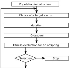
Asynchronous Diﬀerential Evolution (ADE) [5] is a steady state variant of the DE method, its general scheme is shown in Fig. 1. DE uses a populationP of Np vectorsxi to represent candidate solu-tions in the search domain. The initial population is formed by a uniform random sampling of each coordinatexi,jwithin requested initial boundaries [xmin, xmax].

The standard DE is a generational algorithm: mutation and crossover operations are performed for all population members, then as a result of selection DE switches to a next generation. But in a steady state algorithm evolutionary operations are imposed on a selected member of the population, thus a

a_{e-mail: [email protected]}

b_{This work was in part supported by Russian Foundation for Basic Research (Grant No. 13-01-00060).}

(2)

Figure 1: Scheme of a steady-state DE

Table 1: List of ADE variants, used for numerical tests Abbr. Mutation Crossover Pop. sizeNp ACM current-to-pbest ACM inﬂated

RND rand ACM inﬂated

5D current-to-pbest ACM 5D

JADE current-to-pbest JADE 5D

new better vector will take part in evolution without a time lag. In a sequential mode both generational and steady state variants of DE show similar performance in terms of probability of convergence and number of function evaluations to reach the minimum. But for parallel calculations Asynchronous DE exhibits faster speed-up as the number of computing nodes is increased [5].

2.1 Choice of a Target Vector

The choice of atargetvector is a feature which emerges as soon as we switch from a generational algorithm to a steady state variant. In this article we will pick a random member from a population as a target vectorxi. A faster convergence rate can be tried through a choice of either of the worst popu-lation members, thus enforcing replacement of not-so-good candidates. While this choice is proﬁtable for some optimization problems, we found that it reduces the dispersion within the population, and usually leads to a lower probability of convergence to the global minimum. We found that in the case of restart strategies (see Sec. 2.4) the overall performance of ADE weakly depends on a particular choice of the target vector.

2.2 Mutation

In DE amutationvectorvi is constructed by adding to a selected population member a scaled dif-ference vector, which is formed by a simple diﬀerence between randomly picked vectors from the population. In this article we will analyze the following strategies:

‘rand’ [1]: vi=xs+Fi(xr−xq); (2)

‘current-to-pbest’ [3]: vi=xi+Fi(x_bestp −xi)+Fi(xr−xq). (3) Hererand sdenote random members of the population. The index qcorresponds to a randomly selectedxq∈P∪A, with a so-calledarchive A, which storesNpformer population members recently discarded by selection. The indexpis a random index within 0.1Npbest candidates. All vectors in the right sides of Eqs. (2–3) are enforced to be distinct. Thescale factor Fiis sampled for each mutation according to a Cauchy distribution with the location parameterμF and the scale parameter σF = 0.1 [3]. Iﬀ a trial vectorui is selected to replace a target vector xi (see Sec. 2.4), the location parameter is updated

μ

F =(1−cF)μF+cFL2({F}). (4)

HerecF =0.01 is called a learning rate to update the location parameter,L2({F}) is a contraharmonic

(3)

2.3 Crossover

In DE the coordinates of thetrialvectorui,jare picked either from the mutant vectorvi or from the target vectorxi– the so calledcrossoveroperation. We will compare the uniform crossover with the crossover rateCr, adapted by the JADE scheme [3], to a crossover based on an adaptive correlation matrix (ACM) [4].

The coordinates of the trial vectoruiafter uniform crossover are

ui,j=⎧⎪⎪⎨⎪⎪⎩vi,j

rand[0,1)<Cr,ior j=jrand, xi,j otherwise.

(5)

HereCr,i∈[0,1] indicates an average proportion of coordinates selected from the mutant vector into the trial vector. To ensure distinct trial and target vectors, at least one coordinatejrandis taken from the

mutant vector. In JADE the rateCr,iis generated for each crossover according to a normal distribution with the meanμcand the standard deviation 0.1. The meanμcis updated as a result of successful iterations as

μ

c=(1−cμ)μc+cμ{Cr} (6) with a learning factorμc=0.01,{Cr} is a mean over all crossover rates within the current population. While the above JADE scheme treats all coordinates uniformly, ADE with the Adaptive Correla-tion Matrix [4] uses informaCorrela-tion of pairwise correlaCorrela-tions between parameters. The current populaCorrela-tion is used to calculate asample correlation matrix S, its elements read

sjk=

qjk √_q

j jqkk

; qjk= 1

Np−1

i=0

(xi j−x¯j)(xik−x¯k). (7)

Successful stepsare used to cumulatively update an estimation of the correlation matrix – anadaptive

correlation matrix C:

C=(1−c)C+cS. (8)

The coeﬃcientc = 0.01 is alearning ratefor updating the correlation matrix. From the adaptive correlation matrix, the algorithm identiﬁes a group of variables correlated to a selected variablem

{Im}=∀j:|cm j|>cthr, cthr=rand(0,1). (9)

The above set of correlated variables{Im}deﬁnes a subspaceΩmin the search domain. All components of the mutant vectorvi, the indices of which are in the set{Im}, are propagated into a trial vectorui, while other components are taken from the target vectorxi:

ui,j=⎧⎪⎪⎨⎪⎪⎩vi,j

if j∈ {Im}, xi,j otherwise.

(10)

2.4 Selection and Restart

The Diﬀerential Evolution uses a greedy algorithm for the selection: a trial vectorui will replace a target vectorxiiﬀthere is an improvement in corresponding objective function values.

During successive iterations the algorithm analyzes spreads of population members in each co-ordinateΔxjand in the function valuesΔf to avoid stagnation. If at least one of the spreads is too small

∃j Δxj< εxmax

i {|xi,j|}, εx=10

−12 _or _Δ_f _{< ε}

f max i=0,...,Np−1

(4)

an independent restart is initiated [6]. In this work we analyze two restart strategies. One, named ‘5D’, usesNp=5Das a constant population size. Another strategy selectsNminp =10 as an initial size of the population, at each restart the population is increased by a factor 2, if after inﬂation a population size exceeds 20D, an independent restart with the sizeNmin

p is enforced.

3 Numerical Tests

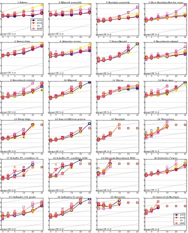
The performance of several variants of ADE-ACM and JADE (Tab. 1) are compared on the set of real-parameter black-box optimization problems BBOB-2015 [7], which is a widely used test bench: more than 100 articles and algorithms have been benchmarked. The test bench contains 24 functions: sepa-rable, non-sepasepa-rable, weakly-structured, unimodal, multimodal, and/or ill-conditioned for dimensions 2, 3, 5, 10, 20 and 40. The performance is measured by the number of successful trials #succ, when an algorithm has reached the function values below f∗+10−8_{, and the}_{expected running time}_ERT(_Δ_f∗₎

to reach values better thanf∗+Δf∗, which is calculated as a ratio of the sum of the evaluations number before the above target value has been reached over the number of successful trials. The maximal number of function evaluations is limited to 106_D_.

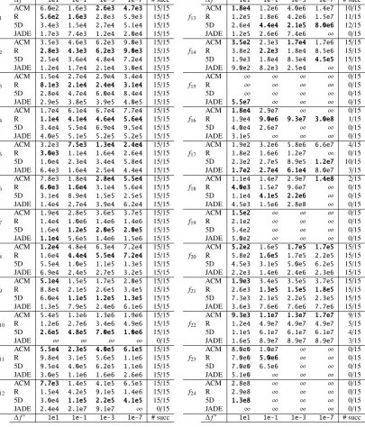
The graphical representation of ERT for all 4 variants is shown in Fig. 2. As the dimension of the problem is increased, ADE-ACM usually performs better than JADE. To exclude differences due to restart procedures, we cite results for ADE-ACM variant ‘5D’ with the fixed population size, which differs from JADE only by the crossover operator. The better performance by ADE-ACM is mainly due to the new crossover, which takes into account the correlations between variables. Convergence rates are presented in Table 2 for the dimensionD = 20. ADE-ACM algorithm solves 17 of 24 functions with probability higher than 0.5 within the allocated number of function evaluations. If restarts are used, both ‘current-to-pbest’ and ‘rand’ strategies have similar performance. For two multimodal functions: Büche-Rastrigin (f4) and Schwefel (f20) ADE-ACM outperforms previously

tested algorithms.

4 Conclusions

In this work we have compared the performance of the recently proposed minimization algorithm of Asynchronous Diﬀerential Evolution with Adaptive Correlation Matrix to the widely used JADE method. By using additional information about linear correlations between variables, which is learned during successful iterations, the new algorithm shows better convergence probabilities and faster con-vergence rates as the dimensionDof the problem exceeds 10. The ADE-ACM can competitively solve a wide range of global optimization problems, both separable, non-separable or partially-separable thanks to the new type of crossover, based on the estimation of the correlation matrix. The new algorithm has a simple structure and is quasi parameter-free from the user’s point of view.

References

[1] K. Price and R. Storn, J. of Global Optimization11, 341–359 (1997) [2] S. Das and P. N. Suganthan, IEEE Trans. Evol. Comput.15, 4–31 (2011) [3] J. Zhang and A.C. Sanderson, IEEE Trans. Evol. Comput.13, 945–958 (2009)

[4] E. Zhabitskaya and M. Zhabitsky, Proceedings of the 15th annual conference on Genetic and evolutionary computation, GECCO’13, ACM, 455–462 (2013)

[5] E. Zhabitskaya and M. Zhabitsky, Lect. Notes in Comp. Sci.7125, 328–333 (2012) [6] E. Zhabitskaya and M. Zhabitsky, Lect. Notes in Comp. Sci.8236, 555–561 (2013)

(5)

2 3 5 10 20 40 0 1 2 3 4

target Df: 1e-8

1 Sphere

ACM RND 5D JADE

2 3 5 10 20 40 0

1 2 3 4

target Df: 1e-8

2 Ellipsoid separable

2 3 5 10 20 40 0 1 2 3 4 5 6

target Df: 1e-8

3 Rastrigin separable

2 3 5 10 20 40 0 1 2 3 4 5 6

target Df: 1e-8

4 Skew Rastrigin-Bueche separ

2 3 5 10 20 40 0

1 2 3 4

target Df: 1e-8

5 Linear slope

2 3 5 10 20 40 0 1 2 3 4 5

target Df: 1e-8

6 Attractive sector

2 3 5 10 20 40 0 1 2 3 4 5 6

target Df: 1e-8

7 Step-ellipsoid

2 3 5 10 20 40 0 1 2 3 4 5 6

target Df: 1e-8

8 Rosenbrock original

2 3 5 10 20 40 0 1 2 3 4 5 6

target Df: 1e-8

9 Rosenbrock rotated

2 3 5 10 20 40 0 1 2 3 4 5 6

target Df: 1e-8

10 Ellipsoid

2 3 5 10 20 40 0 1 2 3 4 5 6

target Df: 1e-8

11 Discus

2 3 5 10 20 40 0 1 2 3 4 5 6

target Df: 1e-8

12 Bent cigar

2 3 5 10 20 40 0 1 2 3 4 5 6 7

target Df: 1e-8

13 Sharp ridge

2 3 5 10 20 40 0 1 2 3 4 5 6 7 8

target Df: 1e-8

14 Sum of different powers

2 3 5 10 20 40 0 1 2 3 4 5 6 7 8

target Df: 1e-8

15 Rastrigin

2 3 5 10 20 40 0 1 2 3 4 5 6 7

target Df: 1e-8

16 Weierstrass

2 3 5 10 20 40 0 1 2 3 4 5 6 7 8

target Df: 1e-8

17 Schaffer F7, condition 10

2 3 5 10 20 40 0 1 2 3 4 5 6 7

target Df: 1e-8

18 Schaffer F7, condition 1000

2 3 5 10 20 40 0 1 2 3 4 5 6 7

target Df: 1e-8

19 Griewank-Rosenbrock F8F2

2 3 5 10 20 40 0 1 2 3 4 5 6

target Df: 1e-8

20 Schwefel x*sin(x)

2 3 5 10 20 40 0 1 2 3 4 5 6 7

target Df: 1e-8

21 Gallagher 101 peaks

2 3 5 10 20 40 0 1 2 3 4 5 6 7

target Df: 1e-8

22 Gallagher 21 peaks

2 3 5 10 20 40 0 1 2 3 4 5 6 7

target Df: 1e-8

23 Katsuuras

2 3 5 10 20 40 0 1 2 3 4 5 6 7 8

target Df: 1e-8

24 Lunacek bi-Rastrigin

ACM RND 5D JADE

Figure 2: Expected running time (as log₁₀value of the number of function evaluations), divided by dimension, for target function valuef∗+10−8_{, versus dimension. Slanted grid lines indicate quadratic}

(6)

Table 2: Expected running time (in number of function evaluations) in the dimensionD=20. Dif-ferent targetΔf∗-values are shown in the top row, #succ is the number of trials that reached the ﬁnal targetf∗+10−8.

Δf∗ 1e1 1e-1 1e-3 1e-7 # succ Δf∗ 1e1 1e-1 1e-3 1e-7 # succ

ACM 6.0e2 1.6e3 2.6e3 4.7e3 15/15 ACM 1.8e4 1.2e6 4.0e6 1.4e7 10/15

f1 R 5.6e2 1.6e3 2.8e3 5.9e3 15/15 f13 R 1.2e5 1.8e6 4.2e6 1.5e7 11/15

5D 3.4e3 1.5e4 2.7e4 5.1e4 15/15 5D 2.6e4 4.4e4 2.1e5 8.0e6 12/15

JADE 1.7e3 7.4e3 1.2e4 2.0e4 15/15 JADE 1.2e5 2.6e6 7.4e6 ∞ 0/15

ACM 3.5e3 4.6e3 6.2e3 9.0e3 15/15 ACM 3.5e2 2.3e3 1.7e4 1.7e6 15/15

f2 R 2.8e3 4.3e3 6.2e3 9.0e3 15/15 f14 R 3.8e2 2.2e3 1.8e4 8.5e6 15/15

5D 2.5e4 3.6e4 4.8e4 7.2e4 15/15 5D 1.9e3 1.8e4 8.3e4 4.5e5 15/15

ACM 1.5e4 2.7e4 2.9e4 3.4e4 15/15 ACM ∞ ∞ ∞ ∞ 0/15

f3 R 8.1e3 2.1e4 2.4e4 3.1e4 15/15 f15 R ∞ ∞ ∞ ∞ 0/15

5D 2.8e4 4.7e4 6.0e4 8.4e4 15/15 5D ∞ ∞ ∞ ∞ 0/15

JADE 2.9e5 3.8e5 3.9e5 4.0e5 15/15 JADE 5.5e7 ∞ ∞ ∞ 0/15

ACM 1.7e4 6.1e4 6.7e4 7.7e4 15/15 ACM 1.8e4 2.9e7 ∞ ∞ 0/15

f4 R 1.1e4 4.1e4 4.6e4 5.6e4 15/15 f16 R 1.9e4 9.0e6 9.3e7 3.0e8 1/15

5D 3.4e4 5.5e4 6.9e4 9.5e4 15/15 5D 4.0e4 2.6e7 ∞ ∞ 0/15

JADE 4.0e5 5.1e5 5.2e5 5.2e5 15/15 JADE 3.1e5 ∞ ∞ ∞ 0/15

ACM 3.2e3 7.5e3 1.3e4 2.4e4 15/15 ACM 1.9e2 3.2e6 5.8e6 6.6e7 4/15

f5 R 3.0e3 1.1e4 1.6e4 2.6e4 15/15 f17 R 1.8e2 1.6e6 1.2e7 ∞ 0/15

5D 1.0e4 2.3e4 3.4e4 5.8e4 15/15 5D 2.3e2 2.7e5 8.9e5 1.2e7 10/15

JADE 6.4e3 1.6e4 2.5e4 4.4e4 15/15 JADE 1.7e2 2.7e4 6.1e4 8.0e7 3/15

ACM 7.8e3 1.8e4 2.8e4 5.5e4 15/15 ACM 1.1e4 1.4e7 2.9e7 1.4e8 2/15

f6 R 6.0e3 1.6e4 3.1e4 5.6e4 15/15 f18 R 4.0e3 1.5e7 9.6e7 ∞ 0/15

5D 3.1e4 8.9e4 1.5e5 2.5e5 15/15 5D 1.1e4 4.1e5 2.2e6 ∞ 0/15

ACM 1.9e4 2.8e5 3.6e5 3.7e5 15/15 ACM 1.5e2 ∞ ∞ ∞ 0/15

f7 R 1.4e4 1.0e6 1.4e6 1.4e6 15/15 f19 R 2.1e2 ∞ ∞ ∞ 0/15

5D 1.6e4 1.2e5 2.0e5 2.0e5 15/15 5D 5.4e2 ∞ ∞ ∞ 0/15

JADE 1.1e4 5.6e5 1.4e6 1.5e6 15/15 JADE 5.0e2 ∞ ∞ ∞ 0/15

ACM 1.2e4 4.8e4 6.3e4 7.2e4 15/15 ACM 5.2e2 1.6e5 1.7e5 1.7e5 15/15

f8 R 1.6e4 4.4e4 5.5e4 7.2e4 15/15 f20 R 5.8e2 1.6e5 1.7e5 2.2e5 15/15

5D 5.5e4 1.0e5 1.1e5 1.3e5 15/15 5D 4.5e3 3.1e5 5.0e5 6.2e5 15/15

ACM _5.1e4 1.5e5 1.7e5 2.0e5 15_/15 ACM _1.9e3 3.4e5 3.5e5 3.7e5 15_/15

f9 R 8.8e4 2.1e5 2.6e5 3.4e5 15/15 f21 R 2.6e3 1.3e5 1.5e5 1.8e5 15/15

5D 6.0e4 1.1e5 1.2e5 1.3e5 15/15 5D 7.3e3 2.1e5 2.2e5 2.3e5 15/15

ACM 5.4e5 1.1e6 1.3e6 1.9e6 15/15 ACM 9.3e3 1.1e7 1.3e7 1.7e7 9/15

f10 R 1.2e6 2.7e6 3.4e6 4.9e6 15/15 f22 R 1.2e4 4.9e7 4.9e7 4.9e7 5/15

5D 2.6e5 4.8e5 7.0e5 1.0e6 15/15 5D 1.1e5 6.1e7 6.1e7 6.1e7 4/15

JADE ∞ ∞ ∞ ∞ 0/15 JADE 1.6e5 8.9e7 8.9e7 8.9e7 3/15

ACM 5.5e4 2.3e5 4.0e5 6.1e5 15/15 ACM 8.0e0 1.0e7 ∞ ∞ 0/15

f11 R 9.8e4 3.1e5 5.6e5 1.1e6 15/15 f23 R 7.0e0 5.0e6 ∞ ∞ 0/15

5D 9.5e4 4.0e5 6.2e5 1.1e6 15_/15 5D 7.0e0 6.5e6 ∞ ∞ 0_/15

JADE 3.0e5 1.1e6 1.6e6 2.6e6 15/15 JADE 5.1e0 ∞ ∞ ∞ 0/15

ACM 7.7e3 1.4e5 4.1e5 6.5e5 15/15 ACM 2.8e8 ∞ ∞ ∞ 0/15

f12 R 1.5e4 4.2e5 9.1e5 1.4e6 15/15 f24 R 2.9e8 ∞ ∞ ∞ 0/15

5D 3.0e4 1.1e5 2.2e5 4.1e5 15/15 5D 1.3e8 ∞ ∞ ∞ 0/15

JADE 2.4e4 2.1e7 9.1e7 ∞ 0_/15 JADE _∞ _∞ _∞ _∞ 0_/15