University of South Carolina
Scholar Commons
Theses and Dissertations
6-30-2016
Ultra-High Temperature Full Field Deformation
Measurements Of Materials Subjected To
Thermo-Mechanical Loading: A DIC Based Study
Guillemo A. Valeri Paoli
University of South Carolina
Follow this and additional works at:https://scholarcommons.sc.edu/etd Part of theAerospace Engineering Commons
This Open Access Thesis is brought to you by Scholar Commons. It has been accepted for inclusion in Theses and Dissertations by an authorized administrator of Scholar Commons. For more information, please [email protected].
Recommended Citation
ULTRA-HIGH TEMPERATURE FULL FIELD DEFORMATION
MEASUREMENTS OF MATERIALS SUBJECTED TO
THERMO-MECHANICAL LOADING: A DIC BASED STUDY
by
Guillermo A. Valeri Paoli
Bachelor of Science Universidad de Los Andes, 2013
Submitted in Partial Fulfillment of the Requirements
For the Degree of Master of Science in
Aerospace Engineering
College of Engineering and Computing
University of South Carolina
2016
Accepted by:
Addis Kidane, Director of Thesis
Michael Sutton, Reader
ii
iii
ACKNOWLEDGEMENTS
I would like to acknowledge Dr. Addis Kidane for his continued guidance
and support throughout the duration of my graduate career. Thanks to his encouragement and advice, I have gained professional experience as an engineer.
Dr. Michael Sutton is acknowledge here for his advice on this work and for
his position as reader and committee member for this thesis. I also thank my respected professors in the department of mechanical engineering for contributing to my academic preparation.
I would like to specially acknowledge Behrad Koohbor for his valuable help
and guidance during my research and course work and particularly for his help in the VFM presented is this work.
This page would be incomplete without the mention of all members of Dr. Kidane’s research group, for their recommendations and company throughout my
research work and my friends and colleagues in mechanical engineering for their moral support and optimism towards my graduate career
Finally, I would like to express my gratitude towards my parents, my
iv
ABSTRACT
Determining the mechanical response of materials at elevated temperatures is a subject of great interest in metal forming, aerospace and
aero-engine industries. For example, measurement of the deformation response under tensile loading at high temperatures is crucial for establishing thermomechanical and thermo-physical properties of materials, consequently, determining the
reliability of a component or structure exposed to elevated temperatures. In order to predict the behavior of materials at ultra-high temperatures, a novel
experimental approach based on Digital Image Correlation (DIC) is proposed and
successfully applied to different materials at temperatures ranging from room temperature to 1100˚C. In these studies, a portable induction heating device
equipped with custom made water-cooled copper coils is used to heat the
specimens. Two different illumination sources along with optical band-pass notch filters, and a stereo-camera configuration system is used to perform 3D-DIC to
analyze stereo-images at a specific temperature.
The effectiveness of the system is demonstrated by successfully performing two different types of experiments; 1) to obtain the coefficient of thermal expansion
(CTE) for two different materials, 309 stainless steel and titanium grade II, as a function of temperature, from room temperature to 1100 ˚C, 2) to study tensile
v
loading at temperatures between 300oC and 900oC. Numbers of experiments are
conducted to study the sensitivity, spatial resolution and repeatability of the DIC measurements. The effect of heat haze on the measurement accuracy is also investigated for this method. Finally, using the temperature and load histories
along with the full-field strain data, a Virtual Fields Method (VFM) based approach is implemented to identify the constitutive parameters governing the plastic
deformation of the material at high temperatures.
Results from these experiments confirm that the proposed method can be
used to measure the full field deformation of materials at ultra-high temperatures subjected to thermo-mechanical loading. Detailed experiment method, analysis
vi
TABLE OF CONTENTS
Acknowledgements ... iii
Abstract ...iv
List of Tables ...viii
List of Figures ...ix
Chapter 1: Introduction ... 1
1.1Displacement and strain measurement... 1
1.2Digital Image Correlation (DIC)... 2
1.3 DIC for High Temperature Applications ... 4
1.4 Objective ... 9
List of References ... 10
Chapter 2: Experimental Method ... 13
2.1 Introduction ... 13
2.2 Equipment used ... 14
2.3 Experimental Procedures ... 26
List of References ... 29
vii
3.1 Introduction ... 30
3.2 Sensitivity analysis ... 30
3.3 Calculation of the Coefficient of Thermal Expansion ... 36
3.4 Summary and Conclusions ... 44
Chapter 4: High Temperature Tensile Response ... 45
4.1 Introduction ... 45
4.2 High Temperature Tensile Test ... 48
4.3 Identification of Visco-Plastic Constitutive Response ... 55
4.4 Results and Discussions ... 61
4.5 Summary and Conclusions ... 68
List of References ... 70
Chapter 5: Sumary and Recommendations ... 72
5.1 Summary ... 72
5.2Recommendations ... 73
viii
LIST OF TABLES
Table 2.2. Induction heater system characteristics... 14
Table 2.3. Cameras specification table... 17
Table 2.4. Technical characteristics o f BP470-55 Blue Bandpass Filter... 19
Table 2.5. Stainless steel 309 chemical components ... 22
Table 2.6. Titanium grade II chemical components ... 22
Table 2.7. Stainless steel 304 L chemical components ... 23
Table 2.8. Flat dog-bone specimen dimensions corresponding to Figure 2.11 ... 24
Table 4.1. Image correlation details used in the present study ... 55
ix
LIST OF FIGURES
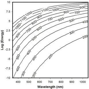
Figure 1.1. Thermal radiation energy as a function of wavelength at various
temperatures ... 7
Figure 2.1. Portable induction heater ... 15
Figure 2.2. Industrial water chiller... 15
Figure 2.3. CEM Infrared Thermometer ... 16
Figure 2.4. Point Grey 5 MP cameras [2] ... 17
Figure 2.5. Variation of radiation energy with respect to temperature for optical wavelengths of (a) 450 nm, (b) 550 nm and (c) 650 nm ... 18
Figure 2.6. BP470 blue bandpass filter wavelength transmission range ... 19
Figure 2.7. (a) Schematic figure of light filtering [3]. (b) Actual optical filter used 20 Figure 2.8. White light illumination set up ... 20
Figure 2.9. Tinius Olsen 5000 tensile testing machine ... 21
Figure 2.10. Stainless steel and titanium specimen dimensions for free expansion tests ... 23
Figure 2.11. Flat dog-bone specimen dimensions ... 24
Figure 2.12. 304 Stainless steel flat dog-bone specimen cut using a CNC water jet... 24
Figure 2.13. Typical high temperature resistant speckle pattern used ... 25
Figure 2.14. Experimental setup used for the CTE calculation tests ... 27
Figure 2.15. Experimental setup for high temperature tensile tests ... 28
x
Figure 3.2. Typical sensitivity analysis experiment ... 32
Figure 3.3. Strain vs temperature under blue light illumination and no fan ... 33
Figure 3.4. Strain vs temperature under blue light illumination with fan... 34
Figure 3.5. Strain vs temperature under white light illumination and no fan... 34
Figure 3.6. Strain vs temperature under white light illumination with fan ... 35
Figure 3.7. Micro strain in the vertical axis vs temperature. Comparison for all tested conditions... 36
Figure 3.8. Full-field vertical and horizontal displacement contours using blue light source... 37
Figure 3.9. Horizontal and vertical shear full-field contours at room temperature (RT), 500 and 1000˚C, using blue light conditions... 38
Figure 3.10. Variation of vertical (εyy) and horizontal (εxx) strains with respect to temperature for 309 Stainless Steel with blue illumination ... 39
Figure 3.11. Variation of vertical (εyy) and horizontal (εxx) strains with respect to temperature for 309 Stainless Steel with white illumination ... 39
Figure 3.12 Variation of vertical (εyy) and horizontal (εxx) strains with respect to temperature for Titanium with blue illumination ... 40
Figure 3.13 Variation of vertical (εyy) and horizontal (εxx) strains with respect to temperature for titanium with white illumination ... 40
Figure 3.14. Variation of CTE with respect to temperature for 309 stainless steel... 42
Figure 3.15. Variation of CTE with respect to temperature for titanium grade II.. 43
Figure 4.1. (a) Tensile specimen geometry with a magnified view of the area of interest and its corresponding gray scale histogram shown in (c). All dimensions in mm. ... 49
Figure 4.2. (a) Experimental setup with a magnification of the area of interest shown in (b)... 51
xi
Figure 4.4. Variation of quantum efficiency of the camera and the transmission efficiency of the utilized band-pass filter as a function of wavelength. ... 54
Figure 4.5. Experimental and model curves obtained at reference temperature (T0
=298 K) and reference strain rate 4.7×10⁻⁴ s-1. ... 56
Figure 4.6. Schematic of the tensile specimen with the dimensions of the area of interest on which full-field measurements are conducted... 58
Figure 4.7. Strain maps showing the distribution of (a) xx and (b) yy over the area of interest at different stress magnitudes (T = 900oC). ... 60
Figure 4.8. Photograph of (a) undeformed and (b) fracture specimen tested at 900oC. Location of the necking zone has been magnified in (c). ... 62
Figure 4.9. Engineering stress-strain curves obtained using cross-head displacement and DIC (T = 900oC) ... 62
Figure 4.10. Experimental stress-strain curves obtained at varying temperatures ... 66 Figure 4.11. Strain rate history curves. ... 67
Figure 4.12. Illustration of the value of the cost function normalized by min. ... 67
1
CHAPTER 1
INTRODUCTION
1.1 DISPLACEMENT AND STRAIN MEASUREMENT
Surface deformation measurement of materials and structures subjected to
mechanical and thermal loading is an important topic in the field of experimental solid mechanics. The importance of these experimental measurements at high temperature deformation is due to their significance in the full-field characterization of thermomechanical and thermophysical properties of various materials. These
materials are used in high temperature applications such as aerospace industries,
high temperature components in aeroengines, automotive, power generation, and high temperature material processes such as, surface treatments, alloying, coatings production, welding, cutting, melting, etc. [10]. The need for an accurate
characterization of the mechanical behavior of materials at high temperatures has led to the development of numerous measurement methods. Aside from the widely
used pointwise strain gauge technique, different full-field non-contact optical
methods, such as speckle interferometry, moiré interferometry , and holography interferometry, and non-interferometric techniques, such as the grid method and
2
require a coherent light source and the measurements need to be conducted in a
vibration-isolated optical platform in the laboratory. Interferometric techniques measure the deformation of the specimen by recording the phase difference of the scattered light wave from the specimen surface before and after deformation. The
measurement results are usually presented in the form of fringe patterns; consequently, further fringe processing and phase analysis techniques are
required to obtain actual displacement results [8]. On the other hand, there have
been efforts in the past two decades to improve non-interferometric full-field measurement techniques such as DIC in the analysis of the thermomechanical
behavior of materials subjected to high temperature deformation [2].
1.2 DIGITAL IMAGE CORRELATION (DIC)
One of the earlier works in the field of image correlation was performed in the
early 1950s by Gilbert Hobrough [9], who compared analog representations of
photographs to register features from various views. Hobrough was able to design and construct an apparatus to correlate high-resolution reconnaissance
photography in order to enable more precise measurement of changeable ground conditions, thus being one of the first investigators to perform image correlation. When digitalized images became more accessible in the 1960s and 1970s,
investigators in robotics and artificial intelligence began to develop vision-based
3
through an explosive growth, meanwhile, the field of experimental solid mechanics
was focused on applying recently developed laser technology to measure deformation: holography, laser speckle, laser speckle photography, and interferometry techniques mentioned before. In 1983, Sutton et al. [1], developed
numerical algorithms and performed preliminary experiments using optically recorded images. In the last decade, 2D-DIC has undergone an immense
worldwide growth; there have been numerous articles using this method since the
year 2000. 2D-DIC requires principally in-plane strains and displacements, and therefore, even small out-of-plane motions will introduce substantial errors in the
deformation measurement. This signifies that 2D-DIC is applicable to plane surfaces only and not on curved surfaces, or the cases where substantial
out-of-plane displacements occur. To resolve this problem, a stereovision system was
developed and employed to make deformation measurements in the late 1990s [9].
Thanks to developments taken place in recent years, three-dimensional digital image correlation (3D-DIC) is now being used for a wide range of time-scales and
length-scales. 3D DIC has been successfully implemented in applications such as:
determining all three components of velocity of imaged fluid particles [11], the use of stereo optical microscopy for deformation and shape measurements on specimen dimensions ranging from a few 300 μm to a few millimeters [15, 20], high
speed imaging systems for use in dynamic stress-strain response (shock loading) [13, 16, 17], measurement of shape and deformation on cylindrical surfaces [17],
4
an area of study for engineered materials like composites [12, 14, 16], and foams
[17] or bio-materials such as biological tissues [18]. In addition, 3D-DIC has been applied on large scale models in civil engineering applications [19] and high temperature deformation measurements, as well [2 - 7]. In particular, high
temperature deformation measurements based on optical methods has been a subject of great interest for the last two decades.
1.3 DIC FOR HIGH TEMPERATURE APPLICATIONS
Determining the material behavior and its properties at high temperatures is a subject of great interest in metal forming, aerospace and aero-engine industries. Measuring the strain and deformation response under tensile loading at high temperatures is crucial for establishing thermomechanical and
thermophysical properties of materials, consequently, determining the reliability of
a component or structure exposed to elevated temperatures.
DIC is probably one of the most appealing techniques for high temperature applications; it has various benefits compared to traditional methods that use
externally applied extensometers, strain gauges or different non-contact optical
methods to measure strain. DIC consists of a simple experimental setup with straightforward specimen preparation. It has the capability to adjust the spatial
resolution, ability to take measurements on curved surfaces and different
5
data, while also, important local variations can be quantified at any area of interest
on the surface; this is the case for heterogeneous materials or at surfaces where the temperature is not constant. It is also applicable to the study both, small and large deformations responses [9].
There have been studies where high temperature DIC was used to measure strains from room temperature up to 2600 ̊C [3]. The first work was performed by
J. S. Lyons et al [2] in 1996. In this study, the authors conducted a series of experiments to assess the ability of DIC to measure full-field surface deformations
at elevated temperatures. For this, a Lindberg furnace, a digital camera with 200 mm lens and white light illumination were used to study the free thermal expansion
strains of an Incoloy 909 specimen and uniform tensile loading of an Inconel 718
specimen. Both specimens where speckled with special ceramic coatings and heated to a maximum temperature of 650 ̊C. In this work, the authors found two
sources of measurement error that caused image distortion: 1. the furnace window, and 2. variations in the refractive index of heated air outside the furnace. The first
problem was solved using an optical quality sapphire furnace window instead of
the standard sapphire window supplied with the furnace. The second problem was solved by implementing a small fan near the furnace window blowing air perpendicular to the camera’s focal axis. The fan mixed the air such that the air
temperature remained constant, not affecting the index of refraction and eliminating the distortion of the specimen’s image. By plotting the strain vs
6
values calculated. Finally, tension tests were performed using a dead-weight
lever-arm system deforming the Inconel 718 specimen with in the elastic region. The results of this work indicated that DIC is capable of measuring thermal and mechanical strains at elevated temperatures (650 ̊C) with the same level of
accuracy as in ambient temperature.
Another limitation found on high temperature DIC, is the visible thermal radiation emitted by the material when heated to temperatures above 650-700 ̊C,
which is brighter than the light source. This black-body radiation alters the contrast
within the surface features (speckles) and makes them very difficult to be interpreted by the correlation routine. The authors [2] suggest using brighter light
and/or filtering the appropriate wavelengths of radiation to allow accurate
measurements at higher temperatures.
Black-body radiation is described by Planck’s equation as a function of
temperature and wavelength.
𝐼(𝜆, 𝑇) =2ℎ𝑐2 𝜆5
1
𝑒𝜆𝑘𝑇ℎ𝑐 − 1
Where, 𝐼(𝜆, 𝑇) is the thermal radiation energy or intensity, h is Planck’s
constant, c is the speed of light, and k is the Boltzmann constant and e is the Euler’s number. By plotting the radiation energy as a function of wavelengths and
temperatures ranging from 200 to 1200 ̊ C, one can observe that as temperature
rises, the emitted thermal radiation includes shorter wavelengths and the radiation
increases rapidly, see next figure.
7
Figure 1.1. Thermal radiation energy as a function of wavelength at various temperatures
Recent works have studied DIC for measuring strains at temperatures ranging from room temperature to 1200 ̊C. Grant et al [4] presented a method that overcomes the black body radiation issue by the implementation of optical filters
and special illumination, providing accurate DIC measurements up to 1100 ̊C. The
experiment consisted of a nickle-based superalloy (RR1000) specimen, with no
applied speckle pattern. The material was loaded under tension and high temperatures, and the Young’s Modulus and CTE were measured. The sample
heating was accomplished by ohmic heating from a current applied across the
8
images taken by one 4M CCD camera. The system required an environmental
chamber to reduce the oxidation by protecting the sample in an argon atmosphere. The results obtained in this work were found to be consistent with values reported by Rolls-Royce plc (RR1000). Grant et al. [4] also found that at temperatures exceeding 800 ̊C, the level of measurement accuracy is deteriorated due to a rapid
oxidation rate. To overcome this issue, the authors proposed the application of a
vacuum chamber for future works. Heat haze was not found to be a problem in this
work [4].
Another limitation associated with the application of DIC at high temperatures is the deteriorating effect of extreme high temperatures to the
speckles on the surface of the specimen. In recent years, the application of novel speckling methods capable of sustaining integrity and efficiency at extreme
temperatures has been studied. Authors have used high temperature resisting
coatings, such as LSI boron nitride and aluminum oxide-based ceramic coatings [2], temperature resistant white Y2O3 paint and other ceramic paints [6], a blend
of black cobalt oxide with liquid commercial inorganic adhesive [5] to form the speckle. Other studies implemented greater resistance techniques, such as using plasma spray for specimen preparation [3], where sprayed tungsten powder was employed at temperatures up to 2600 ̊ C, and finally, the use of the material’s
natural texture as speckle patterns for correlation [4 and 7].
More research is needed to study a simpler high temperature DIC technique for material characterization that overcomes the previously described limitations,
9
machine configurations and for different sample size and geometries, to take
advantage of the convenience of the DIC’s simple and versatile setup equipment.
1.4 OBJECTIVE
The present work focuses on the application and study of a portable novel
3D DIC high temperature measurement system that can be employed on a wide
range of specimen geometries and sizes. In Chapter 2, the experimental methodology, equipment, set up and software used in the experiments are
described. Chapter 3 describes the study and analysis of a specimen subjected to
high temperature free expansion, where High temperature DIC limitations, sensitivity, spatial resolution, and distortion are studied for two different illumination
conditions. The effectiveness of the system is also verified by successfully conducting experiments at temperatures up to 1150˚C and 1000˚C on a 309
stainless steel and titanium specimen, respectively, to determine the variation of
the coefficient of thermal expansion (CTE) as a function of temperature. In Chapter 4 the same portable heating devise is used along with a tensile test machine to
study the thermomechanical properties of a stainless steel 304 specimen, using a novel high temperature speckle technique, blue light LED illumination and a band pass optical filter for image acquisition at temperatures ranging from room temperature (25 ͦ C) up to 900 ͦ C. Finally, the full-field surface measurement results
10 LIST OF REFERENCES
[1] M.A. Sutton, W.J. Wolters, W.H. Peters, W.F. Ranson and S.R. McNeill, 1983, “Determination of Displacements Using an Improved Digital Correlation Method,” Image and Vision Computing, 1(3), pp. 133-139.
[2] J. S. Lyons, J. Liu, and M. A. Sutton, 1996, “High-temperature Deformation Measurements Using Digital-image Correlation,” Experimental Mechanics, 36(1), pp. 64-70.
[3] X. Guo, J. Liang, Z. Tang, B. Cao, and M. Yu, 2014, “High-Temperature Digital Image Correlation Method for Full-Field Deformation Measurement Captured with Filters at 2600 ͦ C using Spraying to Form Speckle Patterns,” Optical engineering,
53(6), pp. 063101-1-12.
[4] B. Grant, H. Stone, P Withers, and M. Preuss, 2009, “High-Temperature Strain Field Measurement using Digital Image Correlation,” Journal of strain analysis for engineering design, 44(4), pp. 263-271.
[5] B. Pan, D. Wu, Z. Wang, and Y. Xia, 2011, “High-Temperature Digital Image Correlation Method for Full-Field Deformation Measurement at 1200 ͦ C,” Measurement Science and Technology, 22, pp. 015701-1-11.
[6] B. Koohbor, G. Valeri, A. Kidane, M. Sutton, 2015, “Thermo-Mechanical Properties of Metals at Elevated Temperatures,” Advancement of Optical Methods in Experimental Mechanics, 3, pp. 117-123.
[7] H. Su, X. Fang, Z Qu, C. Zhang, B. Yan, and X. Feng, 2015, “Synchronous Full-Field Measurement of Temperature and Deformation of C/SiC Composite Subjected to Flame Heating at High Temperature,” Experimental mechanics, DOI 10.1007/s11340-015-0066-5.
11
[9] M A. Sutton, J J. Orteu and H W. Schreier, 2009, Image Correlation for Shape, Motion and Deformation Measurements, Springer. New York, NY.
[10] Yang Y, Li X, Xiao R and Zhang H, 2015, “Digital Image Correlation and Complex Biaxial Loading Tests on Thermal Environment as a Method to Determine the Mechanical Properties of Gh738 using Warm Hydroforming,” High Temperature Material Processes, 19(1), pp. 37-69.
[11] K. D. Hinsch and H. Hinrichs, 1996, “Three-dimensional Particle Image Velocimetry,” Three-Dimensional Velocity and Vorticity Measuring and Image Analysis Techniques, 4, pp. 129-152.
[12] V.P. Rajan, M.N. Rossol and F.W. Zok, 2012, “Optimization of Digital Image Correlation for High-Resolution Strain Mapping of Ceramic Composites,” Experimental Mechanics, 52(9), pp. 1407-1421.
[13] F. Pierron, M.A. Sutton and V. Tiwari, 2011, “Ultra High Speed DIC and Virtual Fields Method Analysis of a Three Point Bending Impact Test on an Aluminum Bar,” Experimental Mechanics, 51(4), pp. 537-563.
[14] B. Koohbor, S. Mallon, A. Kidane and M. A. Sutton, 2014, “A DIC-Based Study of In-Plane Mechanical Response and Fracture of Orthotropic Carbon Fiber Reinforced Composite,” Composites Part B: Engineering, 66, pp. 388–399.
[15] B. Koohbor, S. Ravindran and A. Kidane, 2015, “Meso-Scale Strain Localization and Failure Response of an Orthotropic Woven Glass-Fiber Reinforced Composite,” Composites Part B: Engineering, 78, pp. 308–318.
[16] S. Mallon, B. Koohbor, A. Kidane and M.A. Sutton, 2015, “Fracture Behavior of Prestressed Composites Subjected to Shock Loading: A DIC-Based Study,” Experimental Mechanics, 55(1), pp. 211-225.
[17] B. Koohbor, A. Kidane, W. Lu and M.A. Sutton, 2016, “Investigation of the Dynamic Stress–Strain Response of Compressible Polymeric Foam Using a Non-Parametric Analysis,” International Journal of Impact Engineering, 91, pp. 170–
12
[18] D. Zhang and D.D. Arola, 2004, “Applications of Digital Image Correlation to Biological Tissues,” Journal of Biomedical and Optics, 9(4), pp. 691-699.
[19] R. Ghorbani, F. Matta and M.A. Sutton, 2015, “Full-Field Deformation Measurement and Crack Mapping on Confined Masonry Walls Using Digital Image Correlation,” Experimental Mechanics, 55(1), pp. 227-243.
13
CHAPTER 2
EXPERIMENTAL METHOD
2.1 INTRODUCTION
Before studying the tensile response of materials subjected to high
temperatures using DIC, an analysis of this technique and its effectiveness under elevated temperature conditions is necessary. To do so, experiments were performed where the specimen was continuously heated to 1100 ̊ C under two
different illumination conditions: blue and white light. As mentioned in the objective,
a sensitivity analysis was performed, where the specimen was subjected to free
expansion and 10 images were obtained at different step temperatures and statistically analyzed to determine noise, spatial resolution, distortion and other limitations of this method. The main objective of this experiment was to construct
continuous strain vs temperature plots, calculate the CTE and compare the results using blue and white light with the literature CTE values for two different materials.
This comparison will state the effectiveness of this technique. Also, a test was
performed to study the effect of heat haze in the current experimental setup. Finally, the same experimental setup along with a tensile testing machine, was
14
at temperatures ranging from room temperature up to 900 ̊C. A sensitivity analysis
was also performed for this set up.
2.2 EQUIPMENT USED
All the tests performed in this work were accomplished using the same
equipment and software. However, different materials were employed with
different specimen shape and dimensions.
Heating Source:
Specimens were heated using an Across International IH15 Series Induction Heater [1] equipped with custom-made water-cooled copper coils. The
induction heating system is a portable table-top unit suitable to heat up a wide variety of specimen geometries and sizes and can be employed with different
testing machines, as long as it is equipped with an appropriate coil system. The
following table shows the characteristics of the induction heater used in this study.
Table 2.1. Induction heater system characteristics
Input Voltage 220 VAC single phase
Output Frequency 20 – 80 KHz (mid frequency)
Heating Current 200 – 600 A
15
Figure 2.1. Portable induction heater
Water Chiller
The induction heating system is cooled by an Across International Industrial
Water Chiller that is in charge of maintaining the water that flows through the induction coil at no more than 30 ̊ C. The chiller also cools the power supply and
capacitor of the induction heating system.
16
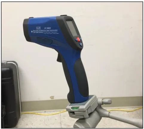
Thermometer
The temperature of the specimen was continuously measured using a
non-contact infrared thermometer facing the center of the specimen, with an accuracy of ±3 ̊ C. The thermometer has a USB port and was connected to a computer to
record the data.
Figure 2.3. CEM Infrared Thermometer
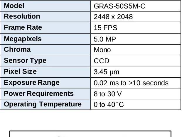
Cameras
A system of two 5 MP Point Grey® stereovision cameras [2] with 100 mm
17
Table 2.2.Cameras specification table
Model GRAS-50S5M-C
Resolution 2448 x 2048
Frame Rate 15 FPS
Megapixels 5.0 MP
Chroma Mono
Sensor Type CCD
Pixel Size 3.45 μm
Exposure Range 0.02 ms to >10 seconds
Power Requirements 8 to 30 V
Operating Temperature 0 to 40 ̊ C
Figure 2.4. Point Grey 5 MP cameras [2]
Optical Filter
It was previously mentioned that the grey-scale intensity of the images will experience a significant change at temperatures above 650 - 700 ̊ C. This can be
shown by plotting once again the radiation energy vs temperature at different wavelengths using Planck’s equation (1). In the next figure, it is noticeable a
remarkable increase in the magnitude of radiation energy as temperature increases beyond T ≈ 700oC. However, the rate of change of the radiation energy
18 0.E+00 1.E+07 2.E+07 3.E+07 4.E+07 5.E+07
0 300 600 900 1200
E
n
e
rg
y
Temperature (oC)
550 nm 0.E+00 1.E+08 2.E+08 3.E+08 4.E+08
0 300 600 900 1200
E
n
e
rg
y
Temperature (oC)
650 nm
for the use of band pass optical filters which allows shorter wavelengths, and also,
additional illumination in order to minimize the unwanted change of grey-scale intensity and increase the level of accuracy in the DIC measurements.
Figure 2.5. Variation of radiation energy with respect to temperature for optical wavelengths of (a) 450 nm, (b) 550 nm and (c) 650 nm
0.E+00 1.E+06 2.E+06 3.E+06
0 300 600 900 1200
E
n
e
rg
y
Temperature (oC)
450 nm
(a)
(b)
19
Consequently, two blue band pass optical filters [3] with a wavelength range
of 435-495 nm were selected and employed in this work. The specifications of the selected filter are shown in the next table and figures.
Table 2.3. Technical characteristics of BP470-55 Blue Bandpass Filter [3]
Wavelength Range 425 – 495 nm
FWHM 85 nm
Tolerance +/- 10 nm
Minimum Peak Transmission > 90%
Surface Quality 40 /20
Compatible LED 450nm, 465nm, 470nm
Figure 2.6. BP470 blue bandpass filter wavelength transmission range 0 10 20 30 40 50 60 70 80 90 100
350 450 550 650 750
20
Figure 2.7. (a) Schematic figure of light filtering [3]. (b) Actual optical filter used
Illumination Source
Two different illumination systems were used: high intensity blue and white
LED illumination.
.
21
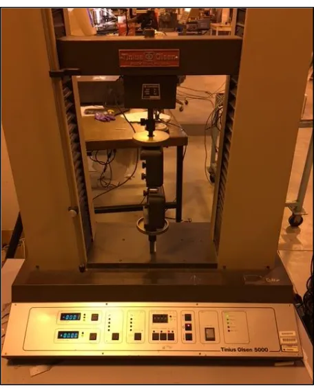
Tensile Testing Machine
Tensile tests were conducted using a Tinius Olsen 5000 tensile testing
machine with a load cell of 20,000 N max load. The tests were performed in displacement control mode and at a constant cross head speed of 10 mm/min,
which is equivalent to a mean strain rate of 2×10⁻³ s-1.
Figure 2.9
.
Tinius Olsen 5000 tensile testing machineSpecimens Characteristics
22
elevated temperatures. The first DIC measurements were performed using a
rectangular fully annealed 309 stainless steel specimen. This material was selected due to its non-magnetic and superior scaling resistance characteristics.
Table 2.4. Stainless steel 309 chemical components [4]
Component Wt. %
Carbon Max 0.2 Chromium 22 – 24 Iron Balance Manganese Max 2
Nickel 12 – 15 Phosphorus Max 0.045
Silicon Max 0.75 Sulphur Max 0.03
A Titanium grade II rectangular specimen was also studied using DIC at high temperatures. This material is widely used in airframe components, cryogenic
vessels and heat exchangers. It is composed of the following elements.
Table 2.5. Titanium grade II chemical components [5]
Component Wt. %
C Max 0.1
Fe Max 0.3 H Max 0.015 N Max 0.03 O Max 0.25
23
Both materials (309 SS and Titanium) were cut to the same size using a
waterjet CNC cutting machine. Two 8mm holes were cut at the edges of the specimens in order to mount them inside the induction coil using two slimmer ceramic rods to allow their free expansion. The next figure shows the dimensions
of the 309 stainless steel and titanium specimens
Figure 2.10. Stainless steel and titanium specimen dimensions for free expansion tests
Finally, low carbon 304 stainless steel flat dog-bone specimens were evaluated under high temperature tensile loading conditions and studied using DIC. It is composed of the following elements.
Table 2.6. Stainless steel 304 L chemical components [6]
Component Wt. %
Carbon Max 0.3 Chromium 18 – 20 Manganese Max 2
Nickel 8 – 12 Phosphorus Max 0.045
24
The as-received stainless steel sheets were cut using a CNC waterjet to the
dimensions showed in the following figure and table.
Figure 2.11. Flat dog-bone specimen dimensions
Table 2.7. Flat dog-bone specimen dimensions corresponding to Figure 2.11
Width 12. mm (0.5 in)
Approx. gage length 88 mm (3.46 in)
Thickness 3.18 mm (0.125 in)
Fillet radius 6.35 mm (0.25 in)
Overall Length 203.2 mm (8 in)
25
Speckle Pattern
All the specimens were coated with a thin layer of ultra-high temperature
resistant white Yttrium Oxide spray paint (max temp: 1500 ̊ C). A high temperature silica-based ceramic paint was then applied on top of the white coating, obtaining
a fine black speckle pattern. The specimens are kept at room temperature to let
the paint fully dry for 24 hours. A typical speckled pattern used is shown in Figure 2.13.
Figure 2.13. Typical high temperature resistant speckle pattern used
Software
26
used to correlate the images and obtain the strains in the area of interest. Finally,
other mathematic tools, such as Matlab, were used to analyze the data and construct the graphs and tables.
2.3 EXPERIMENTAL PROCEDURES
The first experiment type was a sensitivity analysis applied to a 309
stainless steel specimen [8]. For this, the speckled rectangle shaped specimen was held by the two ceramic rods inside the induction coil. Ten images were captured at room temperature before starting the heater. At that moment, the
induction heater was turned on, and heated the specimen until it reached a
maximum temperature of 1000 ̊ C. Ten images were acquired at this temperature and the heater was turned off after a few seconds. As the specimen was cooling down evenly, 10 images were taken every 200 degrees: 1000, 800, 600, 400, 200 ̊
C. This same procedure was done using two illumination conditions, blue and white
light. Each experiment was also repeated using a small table fan blowing air perpendicular to the cameras’ focal axis in order to study the effect of heat haze.
Further details of the sensitivity analysis will be described in Chapter 3. In order to calculate the coefficient of thermal expansion, the specimen was once again heated at a constant rate of 1.6 ̊ C/sec, temperature data and images were taken every 2 seconds (0.5 Hz) until the specimen’s center reached a temperature of
1150 ̊ C and 1000 ̊ C for the 309 stainless steel and titanium specimen,
27
Figure 2.14. Experimental setup used for the CTE calculation tests
Finally, the same experimental setup, along with a tensile testing machine,
was used to study the high temperature tensile response of a speckled flat dog-bone 304 stainless steel specimen and determining its properties. First, the tests
were performed at room temperature (RT) to obtain the reference stress-strain
response of the material using a displacement control mode tensile machine with a constant cross-head speed of 10mm/min. The tensile load is then converted to
true stress. The high temperature tensile tests were performed on a similar manner: The specimen was clamped at the bottom grip of the tensile machine, inside the coil, and heated up to the target temperature, and after waiting several
Wavelength Range
435-495 nm
FWHM
85 nm
Tolerance
+ / - 10 nm
Minimum Peak Transmission
> 90%
Surface Quality
40 / 20
Compatible LED
450 nm, 470 nm
0 10 20 30 40 50 60 70 80 90 100
300 500 700 900 1100
T ra ns mis s ion (% ) Wavelength (nm) IR Thermometer
Specimen Induction
28
minutes for the temperature to become uniform in the area of interest, the
specimen was clamped at the top grip and the experiment immediately initiated (image, load and temperature data acquisition). This test was performed at RT, 300, 500, 700, and 900 ̊ C, using blue light illumination. The temperature history of
the sample at the area of interest was synchronized to record at the same rate as the load and image acquisition. A sensitivity analysis was also performed for this
test set up. This experimental procedure and its parameters are described in
chapter 4 of this thesis. The next figure illustrates this experimental set up.
29 LIST OF REFERENCES
[1] Across International, n.d., from http://www.acrossinternational.com
[2] Point Grey, n.d., from http://www.ptgrey.com
[3] Midwest Optical Systems, n.d., from http://www.midopt.com
[4] AK Steel, n.d., from http://www.aksteel.com
[5] Aerospace Metals, n.d., from http://www.aerospacemetals.com
[6] North American Stainless Steel, n.d., from http://www.northamericanstainless.com
[7] Correlated Solutions, n.d., from http://www.correlatedsolutions.com
30
CHAPTER 3
FREE EXPANSION TEST
3.1 INTRODUCTION
The free expansion experiments were performed for two different materials: 309 stainless steel and titanium grade II. Both specimens were tested using the same equipment and procedure. Chapter 3 describes in detail the analysis, results
and conclusions of two types of experiments: A sensitivity analysis for the stainless steel specimen and the calculation of the coefficient of thermal expansion (CTE)
of both materials. When performing these two experiments it is necessary to
ensure the specimen is free to expand with no constraints, otherwise, a significant internal stress may be produced by the constraints affecting the strain
measurement and ultimately throwing erroneous results. For this, the speckled rectangle shaped specimen was held by two ceramic rods inside the induction coil
which allows the specimen to expand freely in all directions.
3.2 SENSITIVITY ANALYSIS
In order to study the accuracy of the strain measurement at high
temperatures a sensitivity analysis or quantitative error analysis was performed.
31
1000 ̊ C) using white light and blue light separately, and also with fan and with no
fan, as mentioned in the previous chapter. The analysis was performed in a 5 mm diameter circular area in the center of the specimen. The average strains were calculated in the circular area for each of the 10 images on all the step
temperatures. Finally, the strains of the 10 images were averaged and the standard deviation was calculated to visualize the error in the measurement and
compare it for all the temperatures. This same procedure was made for both
illumination cases and with fan and no fan, to study the heat haze phenomenon. The following figure shows the 5 mm circular area of study in the center of the
specimen and also compares the speckle pattern at room temperature with the same at 1000 ̊ C.
Figure 3.1. Specimen at lowest and highest temperature showing the speckle pattern and the 5 mm circular area of study
Speckle pattern at 1000 ̊ C Speckle pattern at room temperature
32
Figure 3.2. Comparison of the speckle pattern with (a) and without the optical filter (b)
The following figure shows a typical strain measurement in temperature
steps, 10 images per temperature.
Figure 3.3. Typical sensitivity analysis experiment 0
0.004 0.008 0.012 0.016 0.02
0 10 20 30 40 50 60
εyy
s
tr
a
in
Number of images 1000 ̊ C
800 ̊ C
600 ̊ C
400 ̊ C
200 ̊ C
25 ̊ C
a
33
It is noticeable in the previous figure that the images were taken during the
cooling phase. The strain in the Y direction is greater at higher temperatures and almost constant at each temperature. The images were used as the input to the DIC software using a subset of 33 pixels and a step size of 11 pixels. The spatial
resolution was calculated to be 26 µm/pix. The next figures show the average strain and standard deviation of the ten images taken at each temperature using
different ilumination and ventilation conditions.
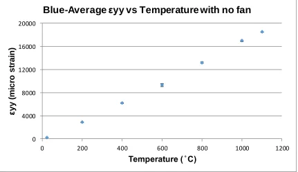
Figure 3.4. Strain vs temperature under blue light illumination and no fan 0
4000 8000 12000 16000 20000
0 200 400 600 800 1000 1200
εy
y
(
m
ic
ro
s
tr
a
in
)
Temperature ( ̊ C)
34
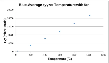
Figure 3.5. Strain vs temperature under blue light illumination with fan
Figure 3.6. Strain vs temperature under white light illumination and no fan 0 4000 8000 12000 16000 20000
0 200 400 600 800 1000 1200
εy y ( m ic ro s tr a in )
Temperature ( ̊C)
Blue-Average
εyy vs Temperature with fan
0 4000 8000 12000 16000 20000
0 200 400 600 800 1000 1200
εy y ( m ic ro s tr a in )
Temperature ( ̊C)
35
Figure 3.7. Strain vs temperature under white light illumination with fan
Figure 3.4 to Figure 3.7, show the results of the analysis for the different conditions. For all cases (blue light, white light, with fan and no fan), a SD of < 3%
of the micro strain was found between the 10 images taken at each temperature;
this indicates the high level of accuracy in the strain measurements of this technique. It is also demostrated that with the use of a blue band pass optical filter, high quality images can be obtained at temperatures up to 1,100 ̊ C, with the use
of either: white light as well as blue light. No specific trend was found that requires
a specific illumination source other than white light. Similarly, it is also conlcuded
that heat haze is not an issue for this experimental set up. The implementation of a fan did not show any improvement or trend in the results; this is due to the fact
that there is no enclosed enviromental chamber in this setup.
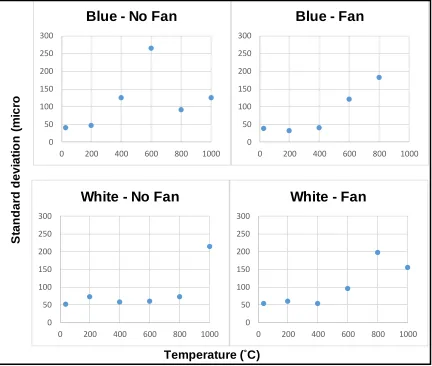
Figure 3.8 compares the standard deviation versus temperature for all conditions.
0 4000 8000 12000 16000 20000
0 200 400 600 800 1000 1200
εy
y
(
m
ic
ro
s
tr
a
in
)
Temperature ( ̊ C)
36
In general, it is noticeable a small increment of SD as the temperature increases,
however the increase is insignificant. In conclusioin, no particular trend is observed for white or blue illumination and/or with and without the use of a fan.
Figure 3.8. Micro strain in the vertical axis vs temperature. Comparison for all tested conditions
3.3 CALCULATION OF THE COEFFICIENT OF THERMAL EXPANSION
Displacement (u and v) full-field contours at different temperatures of the
309 stainless steel specimen, using blue light illumination, are shown in the next 0 50 100 150 200 250 300
0 200 400 600 800 1000
Blue - No Fan
0 50 100 150 200 250 300
0 200 400 600 800 1000
Blue - Fan
0 50 100 150 200 250 300
0 200 400 600 800 1000
White - No Fan
0 50 100 150 200 250 300
0 200 400 600 800 1000
White - Fan
37
figure. This images were taken during the continuous cooling phase of the
specimen every two seconds along with the temperature measurements, and correlated using the same parameters as in section 3.2. Only three temperatures are shown. It is noticeable that the in-plane rigid body motion of translation and
rotation, has been eliminated. Consequently, an equally spaced pattern for horizontal and vertical displacements is clearly demonstrated. The displacement
patterns in the figure, including the displacement magnitude contours, also indicate
a homogeneous thermal expansion.
Figure 3.9. Full-field vertical and horizontal displacement contours using blue light source
Similarly, the strain contours were also plotted and studied. The next figure
demonstrates the horizontal and vertical (εxx and εyy) full-field strain components
0.6 0
-0.6 -0.36 0 0.36 0 0.345 0.69 0.12 0.64 1.16
(mm) (mm) (mm) (µm)
u v (u2+v2)0.5 σ
RT
500oC
38
using the blue illumination condition. It is noticeable a remarkably homogeneous
distribution of both strains. Also, it is observed that the averaged values of εxx and εyyover the entire area of interest, are very similar at 1000˚C (εxx = 0.0192±2% and εyy = 0.0185±2%), this demonstrates the material’s isotropic free thermal expansion
response.
Figure 3.10. Horizontal and vertical shear full-field contours at room temperature (RT), 500 and 1000˚C, using blue light conditions
Finally, strain vs temperature curves were constructed for both illumination
39
Figure 3.11. Variation of vertical (εy y) and horizontal (εxx) strains with respect to
temperature for 309 Stainless Steel with blue illumination
Figure 3.12. Variation of vertical (εy y) and horizontal (εxx) strains with respect to
temperature for 309 Stainless Steel with white illumination 0 0.005 0.01 0.015 0.02 0.025
0 200 400 600 800 1000 1200
S
tr
a
in
Temperature (˚C)
309 Stainles Steel - Blue Illumination
exx [1] - Lagrange
eyy [1] - Lagrange
0 0.005 0.01 0.015 0.02 0.025
0 200 400 600 800 1000 1200
S
tr
a
in
Temperature (˚C)
309 Stainles Steel - White Illumination
exx [cool]
40
Figure 3.13 Variation of vertical (εy y) and horizontal (εxx) strains with respect to
temperature for Titanium with blue illumination
Figure 3.14 Variation of vertical (εy y) and horizontal (εxx) strains with respect to
temperature for titanium with white illumination 0 0.002 0.004 0.006 0.008 0.01
0 200 400 600 800 1000 1200
S
tr
a
in
Temperature (˚C)
Titanium - Blue Illumination
εxx εyy -0.001 0 0.001 0.002 0.003 0.004 0.005 0.006 0.007 0.008 0.009
0 200 400 600 800 1000 1200
S
tr
a
in
Temperature (˚C)
Titanium - White Illumination
exx
41
In the previous figures it is observed that both εxx and εyy evolve in a very
similar way with respect to temperature, this also indicates the isotropic thermal expansion response of both materials.
The coefficient of thermal expansion (α) is calculated by taking the
derivative with respect to the temperature:
𝛼(𝑇) =𝑑𝜀(𝑇) 𝑑𝑇
The best quadratic polynomial was fitted to the ε vs. T graphs shown above, and the derivative was calculated to obtain values of α at each temperature. The quadratic fitted ε vs. T curve shown in the next equation was taken from the
average horizontal and vertical strain vs temperature curve of the 309 stainless steel specimen using white illumination, Figure 3.12.
𝜀(𝑇) = 2.565 ∗ 10−9𝑇2+ 1.481 ∗ 10−5𝑇 − 1.704 ∗ 10−4 30𝑜𝐶 < 𝑇 < 1100𝑜𝐶
After derivation:
𝛼(𝑇) = 2 ∗ 2.565 ∗ 10−9∗ 𝑇 + 1.481 ∗ 10−5
Using the α(T) equation (4), a graph was constructed for each illumination
condition and compared with the literature CTE values for both 309 stainless steel (2)
(3)
42
and titanium from North American Stainless Steel and ASM Material Data sheet,
respectively.
Figure 3.15. Variation of CTE with respect to temperature for 309 stainless steel
Figure 3.15 shows the results in this work compared to the values found in the literature for 309 stainless steel. It is observed that the values obtained in this
work are in good agreement with those found in the literature, with a maximum
difference of about 4% using white light. This small difference might be due to possible differences in the material’s chemical composition, as well as the
experimental methodology conducted to measure the CTE in the literature. 0
5 10 15 20 25
0 200 400 600 800 1000 1200
C
T
E
x
10
-6
(˚C -1 )
Temperature (˚C)
309 Stainless Steel
Blue light
White light
43
The following figure shows the CTE values calculated in this work for both
illumination conditions for titanium grade II. A discrepancy is observed for white light versus blue light. However, it is difficult to compare this values with the published ones in the literature, for the reason that there are discrepancies within
different sources in the literature for this material. This might be because of differences in the chemical composition of the titanium material. At 100˚C the
difference with respect to one literature source (www.swissprofile.com) using blue light is 2%, and at 500 ˚C, the difference is 13 %.
Figure 3.16. Variation of CTE with respect to temperature for titanium grade II 0
2 4 6 8 10 12
0 200 400 600 800 1000 1200
C
T
E
x
1
0
-6
(˚C -1 )
Temperature (˚C)
Titanium
Blue light
44 3.4 SUMMARY AND CONCLUSIONS
The proposed 3D DIC experimental approach was successfully applied to different materials at temperatures ranging from room temperature to 1100˚C. The
use of a blue band pass optical filter provided high quality images at all
temperatures. A standard deviation of < 3% of the micro strain was found between the 10 images taken at each temperature step for all cases (blue light, white light,
with fan and no fan), indicating the high level of accuracy in the strain
measurements of this technique. No particular trend was observed using white or blue illumination and/or with and without the use of a fan; therefore, heat haze is
not a influencing factor for this technique.
In section 3.3 the values of the CTE of two materials: 309 stainless steel and titanium grade II were successfully calculated and compared with the data
available in the literature. A maximum difference of 4% was obtained between the measurements in this work and the values reported in the literature for stainless steel using white light illumination. This difference might be due because of differences in the material’s chemical composition, as well as the experimental
methodology conducted in the literature to measure the CTE of these materials.
It is important to note that the ultra-high temperature resistant Yttrium Oxide white spray paint and the silica-based ceramic black paint, used for the speckle
pattern, remained unaffected for numerous high temperature tests proving its
45
CHAPTER 4
HIGH TEMPERATURE TENSILE RESPONSE
4.1 INTRODUCTION
Determining the mechanical response of materials at elevated
temperatures is a subject of great interest in metal forming, aerospace and aero-engine industries. Measurement of the deformation response under tensile loading at high temperatures is crucial for establishing thermomechanical and thermophysical properties of materials, consequently, determining the reliability of
a component or structure exposed to elevated temperatures. However, there are
certain challenges associated with accurate measurement of high temperature tensile response of materials [1, 2]. Conventionally, high temperature tensile behavior of an engineering material is obtained by conducting tests at well
-controlled environments, and measuring the deformation response using extensometry. Extensometry here can be referred to either contact or non-contact
methods. Although this methodology provides acceptable results and is widely
used in engineering applications, accuracy of the deformation measurements will be highly sensitive to the testing equipment. Moreover, in cases where the
46
quantitative evidence on such deformation localization phenomena. On the other
hand, recently developed temperature-resistant strain gauges provide a more reliable approach for strain measurements performed at significantly high temperatures, with the capability to measure the strain localizations [3]. However,
the application of such temperature-resistant strain gages is limited due to their point measurement capabilities, as well as their maximum working temperature.
Recent advances in the area of non-contact full-field measurements have
proven to provide reliable substitutes for the conventional material testing
methods. In particular, digital image correlation (DIC) is one of the most appealing techniques with the capability of providing accurate information on the deformation
response of materials subjected to extreme conditions, with the benefit of use of straightforward specimen preparation [4]. DIC has the capability to adjust the
spatial resolution, ability to take measurements on curved surfaces [5] and different
specimen sizes and/or shapes [6 – 8] and also the suitability for static and high speed measurements [9, 5]. There have been studies where high temperature DIC
has been used to measure specimen deformation from room temperature up to 2600 ̊C [10]. The first work in this area was performed by J. S. Lyons et al [1] in
1996. In this study, the authors conducted a series of experiments to assess the
capabilities of 2D DIC in the measurement of full-field deformations at elevated
47
pattern, and consequently introduces significant amounts of errors to the image
correlation process. More recent works have studied DIC for measuring strains at temperatures ranging from room temperature to 1200oC. Grant et al [11] presented
a method that overcomes the black body radiation issue by implementation of
optical filters and special illumination sources, providing accurate DIC measurements up to 1100oC.
Another limitation associated with the application of DIC at high
temperatures is due to the deteriorating effect of extreme temperatures on the
speckle pattern. In recent years, the application of novel speckling methods capable of sustaining integrity and efficiency at extreme temperatures has been
studied. Application of temperature-resistant coatings such as LSI boron nitride and aluminum oxide-based ceramic coatings [1], temperature resistant white Y2O3
paint and other ceramic paints [12] a mixture of black cobalt oxide with liquid
commercial inorganic adhesive [2] and the use of plasma sprayed tungsten powder as the speckle pattern are examples on novel speckling methods facilitating the
application of DIC in temperatures up to 2600oC [10].
With the rapidly growing applications of digital image correlation in the area
of material characterization, further research is required to establish simpler high temperature DIC techniques that overcome the previously described limitations. It is also beneficial to devise experimental techniques that employ portable heating
48
focuses on the application of a portable novel high temperature 3D DIC
measurement system that can be employed with a wide range of specimen geometries and sizes. The effectiveness of the system is verified by successfully conducting tensile experiments at temperatures up to 900oC to study the
thermomechanical properties of a 304 stainless steel specimens. The advantage of conducting full-field measurements over the conventional test methodologies
are highlighted in an analytical study based on the method of virtual fields, which
facilitates the identification of the constitutive response of the material with high accuracy.
4.2 HIGH TEMPERATURE TENSILE TEST
4.2.1 Material and Specimen Geometry
Flat dog-bone specimens were extracted from an as-received plate of commercially available low-carbon 304 stainless steel. This material was selected
due to its non-magnetic and superior scaling resistance characteristics. The tensile specimens were coated with a thin layer of ultra-high temperature resistant white paint and a high temperature black silica-based ceramic paint is then applied on
top of the white coating to obtain a fine speckle pattern, used for the image
49
let the paint fully dry. Figure 4.1 illustrates a speckled tensile specimen with a
magnified view of the speckle pattern in the area of interest.
Figure 4.1. (a) Tensile specimen geometry with a magnified view of the area of interest and its corresponding gray scale histogram shown in (c). All dimensions in mm.
4.2.2. Tensile Tests
Tensile tests were first carried out at room temperature to obtain the
reference stress-strain response of the material. To do so, the specimen is inserted into the grips of a conventional tensile frame and pulled to tension in displacement
control mode at a constant cross-head speed of 10 mm/min. The tensile load is
measured by the machine load-cell, and converted to true stress later. True strain and strain rates are determined using the full-field strain data obtained from DIC,
50
To study the high temperature tensile response of the specimens and
determine their properties, the same tensile frame is used. To conduct experiments at high temperatures, an induction heating system was used in conjunction with the tensile frame. The induction heating system employed here is a portable
table-top unit suitable to heat up a wide variety of specimen geometries and dimensions [13] and can be coupled with various testing machines, as long as it is equipped
with an appropriate coil system. The induction heater is equipped with a
water-cooled copper coil system that heats up the specimen at a rate of 1.6oC/s and
provides relatively uniform temperature distribution in the heated area. Prior to the
onset of the tensile experiments, the steel specimen was clamped at the bottom grip of the tensile machine inside the coil and heated up to the target temperature .
After a dwelling time of several minutes allowed for the temperature to become
uniform, the specimen is clamped at the top grip and the test is immediately initiated. Tensile tests are initiated when the specimen temperature reaches the
target temperature. Target temperatures used in this work are 300oC, 500oC,
700oC and 900oC. The temperature of the specimen was measured during the
tensile experiments using a non-contact infra-red thermometer, with a nominal
measurement accuracy of ±3oC. The temperature history of the specimen at the
location of the area of interest was recorded at the same sampling rate used for load and image acquisitions. Reproducibility of the results is ensured by
conducting several tests per target temperature. The next figure illustrates the
51
Figure 4.2. (a) Experimental setup with a magnification of the area of interest shown in (b).
4.2.3. Imaging and Digital Image Correlation
3D digital image correlation was utilized to provide information on the full-field deformation response of the specimens subjected to high temperature
tension. To this purpose, a pair of 5 MP CCD cameras, each equipped with a 100
mm macro lens is used to acquire stereo images during deformation. Images were captured from the area of interest at full-field resolution of 2448×2048 pixel2. The
stereo images were acquired continuously from a 25×12.7 mm2 area of interest
located at the center of the specimen surface (see Figure 4.2-b), at a rate of 1 frame per second. Image acquisition rate was synchronized with the load-cell data
sampling rate via a data acquisition box.
Radiation of a heated object can significantly alter the intensity of the