Modeling and Efficiency Optimization of Steam Boilers by Employing
Neural Networks and Response-Surface Method (RSM)
Heydar Maddah1, Milad Sadeghzadeh2, Mohammad Hossein Ahmadi3, Ravinder Kumar4,
Shahaboddin Shamshirband5,6
1Department of Chemistry, Payame Noor University (PNU), P.O. Box, 19395-3697 Tehran, Iran.
2Department of Renewable Energy and Environmental Engineering, University of Tehran, Tehran, Iran.
3Faculty of Mechanical Engineering, Shahrood University of Technology, Shahrood, Iran.
4School of Mechanical Engineering, Lovely Professional University, Phagwara-144411 Punjab, India
5 Department for Management of Science and Technology Development, Ton Duc Thang University, Ho Chi Minh City, Viet Nam
6Faculty of Information Technology, Ton Duc Thang University, Ho Chi Minh City, Viet Nam
E-mail addresses of the corresponding author:
Abstract
Boiler efficiency is called to some extent of total thermal energy which can be recovered from the fuel.
Boiler efficiency losses are due to four major factors: the dry gas flux, the latent heat of steam in the flue
gas, the combustion loss or the loss of unburned fuel, radiation and convection losses. In this research, the
thermal behavior of boilers in gas refinery facilities is studied and their efficiency and their losses are
calculated. The main part of this research is comprised of analyzing the effect of various parameters on
efficiency such as excess air, fuel moisture, air humidity, fuel and air temperature, the temperature of
combustion gases, and thermal value of the fuel. Based on the obtained results, it is possible to analyze and
make recommendations for optimizing boilers in the gas refinery complex using response-surface method
(RSM).
Keywords: Modeling; Optimization; Steam Boiler; Neural Network; Response-Surface
1. Introduction
Steam boilers are designed to supply steam for heat transfer purposes due to considerable latent heat
value [1,2]. Steam is the main feed of several industries in case of direct or indirect utilization since the heat
transfer coefficient of steam is two times more than water. Therefore, it can be utilized effectively in power
production plants in order to generate electricity [3,4]. Thus, the boiler considered as the most significant
component in power plants, refineries, and so forth [5,6]. The working conditions of a boiler should be
always monitored. It must be highlighted that boilers are working under high temperature and pressurized
status, hence explosion is a serious risk, which is threatening in boilers operation [7,8]. In the design
procedure of the boilers, several aspects, including financial, fuel cost, and maintenance factors should be
covered and noticed. The complexity of steam boiler makes it challenging to perform common measurements
since several factors affect the performance of the boiler. Traditional evaluation methods of boiler
performance are neither cost-effective nor time-saving [9,10]. Besides, to carry out a comprehensive,
accurate analysis, the fuel composition should be analyzed before and after the combustion process in detail
[11,12].
The earlier studies on heat transfer and boiling were carried out by researchers such as Gongur and
Winterton [13] and Kandlikar [14]. The researchers collected a large amount of laboratory data by
conducting several experiments. They achieved to present some correlations that could be employed to
estimate the boiling behavior with little error. In the current time, computational fluid dynamic (CFD)
methods have been used extensively to investigate the boiling regime and its associated involved
mechanisms. Judd and Hwang [15] proposed a model for the prediction of boiling heat, which includes
evaporation and natural heat transfer mechanisms. They found that the evaporation heat transfer is a
significant proportion of the total heat transfer. The application of various CFD models for forced boiling
simulation studied by several researchers [16–20]. Various two-phase models with different simulation
dissolved phase have been used. Also, a series of empirical auxiliary relationships utilized in the simulation
procedure. Krepper et al. [21] provided a model for the evaluation of the boiling mechanism. They
investigated boiling in critical thermal flux conditions. In their research, essential parameters such as
rotation, cross-flow between adjacent channels and bubble concentration regions were determined. By
calculating the temperature of the bar surface, critical areas were identified, and different geometries were
evaluated through CFD modeling. Rivera and Xicale [22] performed experimental evaluation and analytical
assessment on an upstream flow of water-lithium bromide in a uniform vertical heated tube and provided
valuable laboratory data for the saturated nucleate boiling heat transfer coefficients. Owhaib et al. [23]
experimentally and analytically investigated a flow of R-134a fluid in a quartz vertical circular tube which
was uniformly heated by a heater. Their primary purpose was to simulate the saturated and sub-cooled
boiling of the rising refrigerant in the vertical pipe through the pressurized steam that was flowed out of the
pipe. Stevanovic et al. [24] provided a single-dimensional multi-fluid model to predict two-phase flow
patterns in vertical pipes. The presented model was based on the conservation of mass, energy and
momentum and was applicable to any fluid flow that has two-phase flow patterns. Yang et al. [25] presented
numerical simulations and practical experiments for modeling the behavior of the R-141b refrigerant in a
horizontal coil based on the fluid volume method and considering the multiphase flow model. There was a
good agreement between the numerical predictions of phase change with their laboratory data. Kouhikamali
[26] developed a numerical simulation for condensation in a vertical cylinder under the forced convection
regime. Condensation simulations were carried out using fluid volume model and the effects of parameters
such as hydraulic diameter, fluid velocity, Reynolds number, wall temperature difference, and fluid
saturation temperature on heat transfer coefficient were investigated. Ozawa et al. [27]examined a range of
thermal behaviors, including boiling patterns, heat transfer, pressure drop, and critical thermal flux during
high-pressure carbon dioxide boiling for a horizontal microwave channel. The studied variables were tube
diameter changes, mass flux, wall thermal flux, and saturation temperature and pressure of the fluid. Saisorn
et al. [28] examined the R-134a refrigerant evaporation flow through horizontal and vertical mini channels
in order to obtain heat transfer data and also simulation and determination of fluid flow patterns. Dimensions
of the fixed tube were considered to be constant, and the parameters of the thermal flux, mass flux and the
saturation pressure of the inlet fluid were analyzed to determine the flow of fluid in two horizontal and
of parameters such as pressure, mass flux, and thermal flux. Water considered as the working fluid, and the
thermal distribution diagram was plotted near the tube wall. In the following, the effect of the thermal flux
of the wall on the heat transfer coefficient and wall temperature investigated, new experimental correlations
presented, and the heat transfer coefficient compared in a downstream current with a rising flow.
Chen et al. [30] investigated the engineering applications of constructal theory in China. Xie et al. [31]
applied constructal theory to optimize heat transfer performance and pressure drop of an evaporator boiler.
Behbahaninia et al. [32] presented a novel auditing approach to monitoring the performance of steam boilers
based on exergy approach. This method was proposed based on ASME ptc 4.1 to calculate the exergy loss
and exergy efficiency. Some significant factors such as exergy destruction inside the boiler, exergy loss in
the wall of the boiler, exergy destruction in the gas-air heater, exergy loss in the flue gas. It concluded that
the major irreversibility of the boiler is due to inside exergy destruction, i.e. more than 38%. In addition, the
total exergy efficiency of the boiler was calculated by 53.7%. Li et al. [33] investigated the performance of
a boiler in a biomass energy production plant and used the exergy method. It was reported that the most
irreversibilities was originated from the combustion process. It was found that the total exergy efficiency of
the boiler could be increased by decreasing the excess air and by augmenting the superheater temperature.
Li et al. [34] compared various scenarios in order to prevent the inefficient working of a boiler in a 660 MW
coal power plant. The authors recommended that the approach of closing part of the 2nd air nozzle was the
most beneficial approach among other studied methods. In another study, Li et al. [35] analyzed the effect
of increasing primary air ratio on the performance of a boiler in a coal-fired power plant. It was monitored
that increasing the primary air temperature was more practical and also improved the thermal performance
of the boiler instead of rising the air ratio. Javan et al. [36] performed an exergoeconomic optimization of a
gas-fired steam power plant by applying a genetic algorithm. Based on the results, the boiler was the most
exergy destructive source in the power plant. Therefore, two approaches presented and compared to decrease
the amount of exergy destruction in the boiler in order to improve the total efficiency of the power plant:
reducing the amount of excess air and decreasing the outlet temperature of the boiler's exhaust gas through
heat recovery approaches. It was stated that this optimization technique was able to lower the total cost rate
by 20% and decreased the dangerous environmental impact by 88%. Pattanayak et al. [37] optimized the
sootblowing frequency of a boiler in a coal-fired power plant in order to lower the hazardous combustion
the efficiency of a steam boiler. Nikula et al. [39] proposed a data-driven model to estimate and monitor the
thermal performance of the boiler in order to achieve a higher efficiency boiler with a reduction in emission
pollutants. Vandani et al. [40] used a genetic algorithm and partial swarm optimization techniques to improve
the exergetic efficiency of boiler blowdown. It was stated that outlet pressure and outlet temperature of the
boiler played a significant role in improving the exergy efficiency.
In this research, the modeling of boiler efficiency will be performed based on experimental data and
response-surface method (RSM). Steam flow rate and output temperature selected as independent variables.
The dependent variable is considered as the boiler efficiency.
2. Modeling Fundamentals
The neural network model is a data-driven model, so it requires experimental data to build the model.
In this study, with the help of the neural network modeling, the target output is predicted through two input
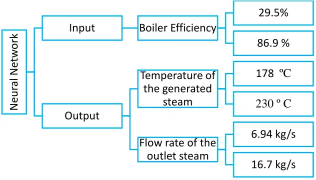
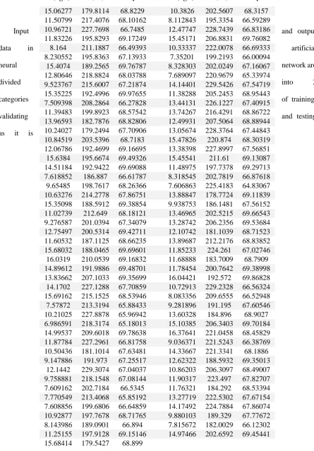
data sets. Figure 1 illustrates the upper and lower limit of input and output data. The utilized input data in
the neural network modeling process is listed in Table 1. Where, 𝑚̇ represents the mass flow rate (kg/s), T
is the temperature (ºC), and η states the boiler efficiency.
Figure 1. The upper and lower limit of input and output data for construction of a neural network model
N
eu
ral
N
et
w
or
k
Input
Boiler Efficiency
29.5%
86.9 %
Output
Temperature of
the generated
steam
178 ºC
230 º C
Flow rate of the
outlet steam
6.94 kg/s
Table 1. The experimental data used to form the neural network model
Input and output
data in artificial
neural network are
divided into 3
categories of training,
validating and testing
as it is
𝐦̇(kg/s) T(ºC) η 𝐦̇(kg/s) T(ºC) η
15.06277 179.8114 68.8229 10.3826 202.5607 68.3157 11.50799 217.4076 68.10162 8.112843 195.3354 66.59289 10.96721 227.7698 66.7485 12.47747 228.7439 66.83186 11.83226 195.8293 69.17249 15.45171 206.8831 69.76082 8.164 211.1887 66.49393 10.33337 222.0078 66.69333 8.230552 195.8363 67.13933 7.35201 199.2193 66.00094 15.4074 189.2565 69.76787 8.328303 202.0249 67.16067 12.80646 218.8824 68.03788 7.689097 220.9679 65.33974 9.523767 215.6007 67.21874 14.14401 229.5426 67.54719 15.35225 192.4996 69.97655 11.38288 205.2453 68.95443 7.509398 208.2864 66.27828 13.44131 226.1227 67.40915 11.39483 199.8923 68.57542 13.74267 216.4291 68.86722 13.96593 182.7876 68.82806 12.49931 207.5064 68.88944 10.24027 179.2494 67.70906 13.05674 228.3764 67.44843 10.84519 203.5396 68.7183 15.47826 220.874 68.30319 12.06786 192.4699 69.16695 13.38398 227.8997 67.56851 15.6384 195.6674 69.49326 15.45541 211.61 69.13087 14.51184 192.9422 69.69088 11.48975 197.7378 69.29713 7.618852 186.887 66.61787 8.318545 202.7819 66.87618 9.65485 198.7617 68.26366 7.606863 225.4183 64.83067 10.63276 214.2778 67.86751 13.88847 178.7724 69.11839 15.35098 188.5912 69.38854 9.938753 186.1481 67.56152 11.02739 212.649 68.18121 13.46965 202.5215 69.66543 9.276587 201.0394 67.34079 13.28742 206.2356 69.53684 12.75497 200.5314 69.42711 12.10742 181.1039 68.71523 11.60532 187.1125 68.66235 13.89687 212.2176 68.83852 15.68032 188.0465 69.69601 11.85233 224.261 67.02746 16.0319 210.0539 69.16832 11.68888 183.7009 68.7909 14.89612 191.9886 69.48701 11.78454 200.7642 69.38998 13.83662 207.1033 69.35699 16.04421 192.572 69.86828 14.1702 227.1288 67.70859 10.72913 229.2328 66.56324 15.69162 215.1525 68.53946 8.083356 209.6555 66.52948 7.57872 213.3194 65.88433 9.281896 191.195 67.60546 10.21025 227.8878 65.96942 13.60328 184.896 68.9027 6.986591 218.3174 65.18013 15.10385 206.3403 69.70184 14.99537 209.6018 69.78638 16.37641 221.0458 68.45829 11.87784 227.2961 66.81758 9.036371 221.5243 66.38769 10.50436 181.1014 67.63481 14.33667 221.3341 68.1886 9.147886 191.973 67.25517 12.62322 188.5932 69.35013
demonstrated in Figure 2. Training data is used to create a model. The validation data is used to check the
quality and correctness of the training stage. Test data is not used in the training phase and is used only for
performance evaluation and examining the neural network modeling.
Figure 2. Randomized classification of empirical data in order to construct a neural network model
Figure 3. Triple layer neural network structure
The neural network is expressed on the basis of a particular topology. The topology is referred to the
structure of the network. In this investigation, a triple layer neural network, Figure 3, is used to predict the
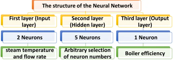
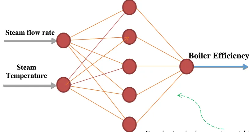
output variable, the boiler efficiency. A sample 2-5-1 structure is depicted in Figure 4. As can be seen, the
number of neurons in the first, second and third layers is 2, 5, and 1, respectively. The number of neurons in
the second layer, known as the hidden layer, is arbitrary. In this research, 5 neurons are determined to be
placed in the hidden layer. The selection the neurons' number in the first and third layers is not arbitrary and
is selected based on the number of input data to the model. According to Figure 4, the neurons in each layer
are connected by the edges to the neurons in the adjacent layer. These edges determine the relationship
between the input and output variables by the weight coefficients assigned to them. This mathematical
relation is discussed in the following.
Number of Inputs (93 data)
Test Data
15%
14 data
Validation Data
15%
14 data
Training Data
70%
67 data
The structure of the Neural Network
First layer (Input
layer)
2 Neurons
steam temperature
and flow rate
Second layer
(Hidden layer)
5 Neurons
Arbitrary selection
of neuron numbers
Third layer (Output
layer)
1 Neuron
Figure 4. Sample schematic structure of a 2-5-1 neural network model: 2 neurons in the input layer, 5
neurons in the hidden layer, and a neuron in the output layer
The connection between input data and output data is determined by a network of linked nodes as shown
in Figure 4.
Input and output data are correlated with a series of weighted coefficients. There are 10 (2*5=10) edges
between the first layer and the second layer. There are 5 (5*1=5) edges between the second layer and the
third layer. Each edge is assigned a weight. The weights of these edges are presented as a 5× 2 matrix and a
5 × 1 matrix. The relationship between output and input data is expressed as follows:
( 1 ) 𝜂 = [𝐿𝑊]1×5× 𝑡𝑎𝑛ℎ ( [𝐼𝑊]5×2× [𝑚̇𝑇]
2×1+ [𝑏1
]5×1 ) + [𝑏2]1×1
Neural network edges carrying weight
Boiler Efficiency
Steam
The employed variables in the Eq. (1) are listed and defined in Table 2.
Table 2. Definition of required variables in modeling using neural network
Variable Definition Description
𝜼𝑵𝑵 Output of the neural
network model
Boiler efficiency, the final output of the neural network
model
𝒎̇ 1st input variable Steam mass flow rate, Kg/s
𝑻 2nd input variable Temperature, ℃
[𝑰𝑾]𝟓×𝟐 Edge matrix between 1st
and 2nd layers
Each of the edges between layer 1 and 2 is assigned a
weight
[𝑳𝑾]𝟏×𝟓 Edge matrix between 2nd
and 3rd layers
Each of the edges between layer 2 and 3 is assigned a
weight
[𝒃𝟏]𝟓×𝟏 Bias matrix of the 2nd layer After multiplying the weight matrix in the input signal, the
results are summed with the bias.
[𝒃𝟐]𝟏×𝟏 Bias matrix of the 3rd layer After multiplying the weight matrix in the input signal, the
results are summed with the bias.
3. Modeling Results of Boiler Efficiency Using Neural Network
In this section, the obtained results from the modeling by means of neural network are compared with
the actual results. The total number of data used in modeling is 95. Of these, 70% are for training, 15% for
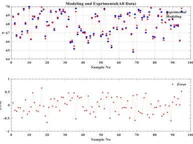
validating, and the rest for testing the network. Figure 5 illustrates the graph error of the modeling results.
Figure 5. Comparison of model estimations with actual efficiency measurements (95 Data)
As it is monitored, the prediction error is approximately 1% in the positive and negative range with the
help of the neural network. In the following figures, the actual data (experimental) and modeling data are
presented separately for each of the three categories, i.e. categories of training, validating, and testing.
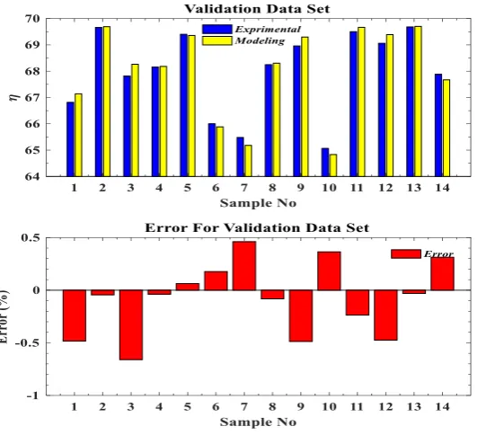
Figure 7. Comparison of experimental data and modeling for validation (14 data)
Figures 6-8 demonstrate the error in the modeling data in percent for the three classes of train,
validation, and test, respectively. Based on these figures, the error data for training, validating, and testing
phases are obtained by 0.6, 0.5, and 1, respectively. Test data are not involved in the training stage. Therefore,
test data error is more than training and validation.
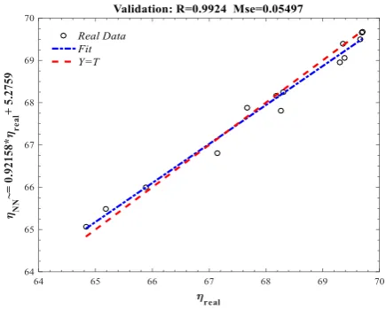
The regression line diagram along with the mean squared error (MSE) and correlation coefficient for
each of categories of training, validation, and test are shown in Figures 9-11. As it is expected, the low error
rate and high correlation coefficient indicate the proper performance of the neural network in prediction of
the boiler efficiency. In the Figures 9-11, horizontal axis is real efficiency and vertical axis demonstrates the
modeling efficiency. Ideally, when the model error is zero, all points are located on the line Y = T (First
bisector quadrant line). In reality there is a small amount of error that causes the points to be scattered up
and down the line. The best-passing equation from the points in this graph along with the correlation
coefficient as well as the MSE error are given in the following figures for the train, validation, and test stages.
Figure 9. The regression line diagram for training data
Figure 11. The regression line diagram for test data
The network performance in respect to modeling error and regression coefficient R2 are obtained
according to Table 3.
Table 3. The performance of the neural network in predicting efficiency
Train (70%) Validation (15%) Test (15%)
Number of data 67 14 14
Mean Squared Error
(MSE)
0.033 0.055 0.069
Regression coefficient
(R2)
0.998 0.994 0.966
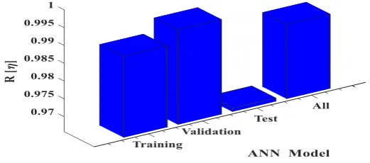
The performance values (error and correlation coefficient) of the network are graphically depicted in
Figure 12 and Figure 13, respectively, as follows:
Figure 13. Correlation coefficient of training, validation, test, and all.
Most of the stopping training criteria are based on the mean square error control. Therefore, the MSE
curve is plotted as a function of the repetition of the training algorithm in Figure 14.
Monitoring MSE for test data and validation data is performed in the same way as training data in
various repetitions, and when the validation data error begins to increase, the training should be stopped.
The most generalization is occurred at the 11th epoch.
Figure 14. Mean Squared Error Diagram in Different epochs of Training Process for estimating the Boiler
Efficiency.
The mean square error (MSE) during the training process is demonstrated in the Figure 14. Obviously,
increasing the frequency is led to gradually decrease in error of all three categories. With the progress of the
algorithm in each repetition, the mean square error for the validation data is calculated. The algorithm will
not stop until the validation error decreases, and training continues. When the validation error is not
is adjustable in the software. This number is known as the validation check and is assumed 6 by default in
the software.
The point where the validation error reaches its minimum is considered as the output of the model. For
instance, in the Figure 14 before the 11th epoch, the network error trend for the training, validation, and
testing data is decreasing and from repetition 11, the verification error is increasing, while the training data
error continues to decline. From Repeat 11 to Repeat 17 (6 consecutive repetitions), the validation error has
an increasing trend, so the training algorithm ends and Repeat No. 11 is considered as an output. In other
words, the training is stopped if the evaluation set error is raised in 6 consecutive repetitions. This stop
occurred at repeat No. 11. It should be noted that the algorithm calculates the mean squared error as follows:
( 2 )
𝑀𝑆𝐸 = ∑(𝜂𝑁𝑁− 𝜂𝑅𝑒𝑎𝑙)
2
𝑁𝑒
𝑛
𝑖=1
In Eq. (2), 𝜂𝑁𝑁 denotes the obtained modeling efficiency, 𝜂𝑅𝑒𝑎𝑙 indicates the real measured boiler efficiency,
and Ne represents the total number of samples.
4. Optimization with the Help of the Response-Surface Method
Response-surface method or RSM is a collection of statistical techniques and applied mathematics for
creating empirical models. The purpose of response-surface is to optimize the response (output variable),
which is influenced by several independent variables (input variables). In this study, two independent
variables of flow rate and output steam temperature of the boiler, and dependent variable of efficiency are
discussed.
In Figure 15, the fitted response surface on the boiler experimental data is presented, and as can be
seen, this surface is well suited with the experimental data. The constant coefficients obtained from the
RSM optimization for Eq. (3) are presented in the Table 4.
Figure 15. RSM analysis (inputs: flow rate and temperature)
Table 4. The optimal values of the constants which are obtained by RSM optimization
Constants C0 C1 C2 C12 C11 C22
Optimized
Value
-31.372 1.690 0.8977 -0.00047 -0.05112 -0.00227
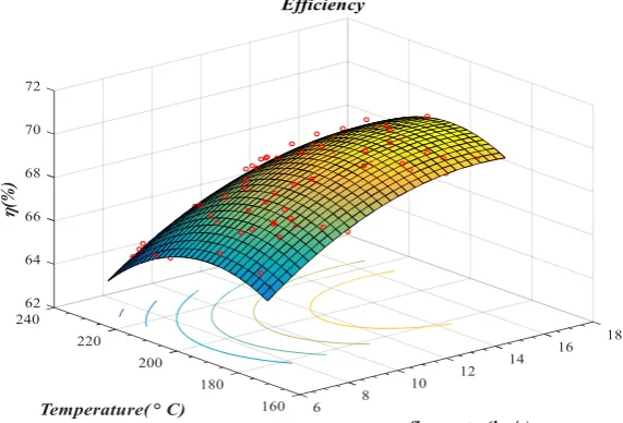
In Figure 16, the response surface along with the experimental data is presented in a 3-D graph.
Figure 16. The fitted surface on the empirical data obtained from the boiler
Table 5. The optimal boiler efficiency (obtained from the RSM)
Variable Objective function 1st independent
variable
2nd independent
variable
Unit Efficiency (%) Flow rate (kg/s) Temperature (℃)
Optimal value from RSM 69.8 15.7 195.9
5. Sensitivity Analysis of Effecting Variables
With the aid of sensitivity analysis, the effect of each independent variable can be obtained on dependent
variables (boiler efficiency). In the sensitivity analysis, all variables are assumed to be constant and only one
variable within its permitted range is changed. In Figure 17, sensitivity analysis is performed for the
temperature variable. As can be monitored, the magnitude of the efficiency at 196 ° C results to its maximum
value for almost all flow rates. As the flow rate increases and becomes close to the designed flow rate of the
boiler changes, the rate of change in efficiency will be slower in terms of temperature.
Figure 17. Temperature sensitivity analysis at four different flow rates
Figure 18 shows the sensitivity analysis for the flow rate independent variable. As can be seen, in the
flow rate of 15.7 Kg /s, the amount of efficiency yields to its maximum. With increasing temperature, first,
Figure 18. Flow rate sensitivity analysis at four different temperatures
7. Conclusion
The plant's steam production and distribution unit is designed and installed by Iranian Energy
Engineering Company "Garmagostar" in order to provide steam and heating loads of reboilers, heaters,
flares, sweetening packages, seawater treatment plant and other steam utilities. The total number of data used
in the modeling process is 95 which are categorized as 70% for training, 15% for validation, and the rest for
test procedure of the network. Modeling by means of neural network yields to the prediction error in the
range of ∓1. The associated error of the training stage, validation stage, and test stage were obtained less
than 0.6%, 0.5%, and 1%, respectively. As expected, the data test error is higher than training and validation
due to the lack of participation of the test data at the training and learning stage of the neural network. In the
ideal mode, when the model error is zero, all points are placed on the line of Y = T (Bisection of 1st and 3rd
coordination sections). In practice there is a small amount of error that causes the points to be scattered up
and down of the line. The best-passing equation of the points along with the correlation coefficient as well
as the mean square error are calculated for validation and test phases of the total data. Response-surface
method (RSM) is a set of statistical techniques and applied mathematics for constructing empirical models.
The target goal of the RSM is to optimize the response (output variable), which is influenced by several
independent variables (inputs). In this study, two independent variables of steam flow rate and temperature
temperatures of 196 ° C results in maximum efficiency for almost all flow rates. As the flow rate increases
and approaches to the specific boiler design flow rate, the trend of variations of efficiency in term of
temperature is getting slower. Also, sensitivity analysis for the flow rate variable was performed and it is
monitored that the maximum amount of efficiency is yielded at flow rate of 15.7 Kg/s. With increasing
temperature, first, the efficiency increases and then decreases.
References
[1] Echi S, Bouabidi A, Driss Z, Abid MS. CFD simulation and optimization of industrial boiler. Energy
2019;169:105–14. doi:10.1016/J.ENERGY.2018.12.006.
[2] Ahmadi MH, Alhuyi Nazari M, Sadeghzadeh M, Pourfayaz F, Ghazvini M, Ming T, et al.
Thermodynamic and economic analysis of performance evaluation of all the thermal power plants: A
review. Energy Sci Eng 2019;7:30–65. doi:10.1002/ese3.223.
[3] Szega M, Czyż T. Problems of calculation the energy efficiency of a dual-fuel steam boiler fired with
industrial waste gases. Energy 2019;178:134–44. doi:10.1016/J.ENERGY.2019.04.068.
[4] Mohammadi A, Ashouri M, Ahmadi MH, Bidi M, Sadeghzadeh M, Ming T. Thermoeconomic analysis
and multiobjective optimization of a combined gas turbine, steam, and organic Rankine cycle. Energy
Sci Eng 2018:506–22. doi:10.1002/ese3.227.
[5] Hajebzadeh H, Ansari ANM, Niazi S. Mathematical modeling and validation of a 320 MW tangentially
fired boiler: A case study. Appl Therm Eng 2019;146:232–42.
doi:10.1016/J.APPLTHERMALENG.2018.09.102.
[6] Shams Ghoreishi SM, Akbari Vakilabadi M, Bidi M, Khoeini Poorfar A, Sadeghzadeh M, Ahmadi MH,
et al. Analysis, economical and technical enhancement of an organic Rankine cycle recovering waste
heat from an exhaust gas stream. Energy Sci Eng 2019:1–25. doi:10.1002/ese3.274.
[7] El Hefni B, Bouskela D. Boiler (Steam Generator) Modeling. Model. Simul. Therm. Power Plants with
ThermoSysPro A Theor. Introd. a Pract. Guid., Cham: Springer International Publishing; 2019, p. 153–
64. doi:10.1007/978-3-030-05105-1_7.
[8] Sankar G, Kumar DS, Balasubramanian KR. Computational modeling of pulverized coal fired boilers –
[9] Trojan M. Modeling of a steam boiler operation using the boiler nonlinear mathematical model. Energy
2019;175:1194–208. doi:10.1016/J.ENERGY.2019.03.160.
[10] Naeimi A, Bidi M, Ahmadi MH, Kumar R, Sadeghzadeh M, Alhuyi Nazari M. Design and exergy
analysis of waste heat recovery system and gas engine for power generation in Tehran cement factory.
Therm Sci Eng Prog 2019;9:299–307. doi:10.1016/j.tsep.2018.12.007.
[11] Barroso J, Barreras F, Amaveda H, Lozano A. On the optimization of boiler efficiency using bagasse as
fuel☆. Fuel 2003;82:1451–63. doi:10.1016/S0016-2361(03)00061-9.
[12] Said SM, Hamouda AS, Mahmaoud H, Abd-Elwahab S. Computer-based boiler efficiency
improvement. Environ Prog Sustain Energy 2019:1–9. doi:10.1002/ep.13161.
[13] Gungor KE, Winterton RHS. A general correlation for flow boiling in tubes and annuli. Int J Heat Mass
Transf 1986;29:351–8. doi:10.1016/0017-9310(86)90205-X.
[14] Kandlikar SG. A General Correlation for Saturated Two-Phase Flow Boiling Heat Transfer Inside
Horizontal and Vertical Tubes. J Heat Transfer 1990;112:219–28.
[15] Judd RL, Hwang KS. A Comprehensive Model for Nucleate Pool Boiling Heat Transfer Including
Microlayer Evaporation. J Heat Transfer 1976;98:623–9.
[16] Krepper E, Rzehak R. CFD for subcooled flow boiling: Simulation of DEBORA experiments. Nucl Eng
Des 2011;241:3851–66. doi:10.1016/J.NUCENGDES.2011.07.003.
[17] Kunkelmann C, Stephan P. CFD simulation of boiling flows using the volume-of-fluid method within
OpenFOAM. Numer Heat Transf Part A Appl 2009;56:631–46. doi:10.1080/10407780903423908.
[18] Zhang X, Yu T, Cong T, Peng M. Effects of interaction models on upward subcooled boiling flow in
annulus. Prog Nucl Energy 2018;105:61–75. doi:10.1016/J.PNUCENE.2017.12.004.
[19] Promtong M, Cheung SCP, Yeoh GH, Vahaji S, Tu J. CFD investigation of sub-cooled boiling flow
using a mechanistic wall heat partitioning approach with Wet-Steam properties. J Comput Multiph
Flows 2018;10:239–58. doi:10.1177/1757482X18791900.
[20] Pothukuchi H, Kelm S, Patnaik BSV, Prasad BVSSS, Allelein H-J. Numerical investigation of
2018;129:1604–17. doi:10.1016/J.APPLTHERMALENG.2017.10.105.
[21] Krepper E, Končar B, Egorov Y. CFD modelling of subcooled boiling—Concept, validation and
application to fuel assembly design. Nucl Eng Des 2007;237:716–31.
doi:10.1016/J.NUCENGDES.2006.10.023.
[22] Rivera W, Xicale A. Heat transfer coefficients in two phase flow for the water/lithium bromide mixture
used in solar absorption refrigeration systems. Sol Energy Mater Sol Cells 2001;70:309–20.
doi:10.1016/S0927-0248(01)00073-3.
[23] Owhaib W, Palm B, Martín-Callizo C. Flow boiling visualization in a vertical circular minichannel at
high vapor quality. Exp Therm Fluid Sci 2006;30:755–63.
doi:10.1016/J.EXPTHERMFLUSCI.2006.03.005.
[24] Stevanovic V, Prica S, Maslovaric B. Multi-Fluid Model Predictions of Gas- Liquid Two-Phase Flows
in Vertical Tubes. FME Trans 2007;35:173–81.
[25] Yang Z, Peng XF, Ye P. Numerical and experimental investigation of two phase flow during boiling in
a coiled tube. Int J Heat Mass Transf 2008;51:1003–16.
doi:10.1016/J.IJHEATMASSTRANSFER.2007.05.025.
[26] Kouhikamali R. Numerical simulation and parametric study of forced convective condensation in
cylindrical vertical channels in multiple effect desalination systems. Desalination 2010;254:49–57.
doi:10.1016/J.DESAL.2009.12.015.
[27] Ozawa M, Ami T, Umekawa H, Matsumoto R, Hara T. Forced flow boiling of carbon dioxide in
horizontal mini-channel. Int J Therm Sci 2011;50:296–308.
doi:10.1016/J.IJTHERMALSCI.2010.04.017.
[28] Saisorn S, Kaew-On J, Wongwises S. An experimental investigation of flow boiling heat transfer of
R-134a in horizontal and vertical mini-channels. Exp Therm Fluid Sci 2013;46:232–44.
doi:10.1016/J.EXPTHERMFLUSCI.2012.12.015.
[29] Shen Z, Yang D, Chen G, Xiao F. Experimental investigation on heat transfer characteristics of smooth
tube with downward flow. Int J Heat Mass Transf 2014;68:669–76.
[30] Chen L, Feng H, Xie Z, Sun F. Progress of constructal theory in China over the past decade. Int J Heat
Mass Transf 2019;130:393–419. doi:10.1016/J.IJHEATMASSTRANSFER.2018.10.064.
[31] Xie Z, Feng H, Chen L, Wu Z. Constructal design for supercharged boiler evaporator. Int J Heat Mass
Transf 2019;138:571–9. doi:10.1016/J.IJHEATMASSTRANSFER.2019.04.078.
[32] Behbahaninia A, Ramezani S, Lotfi Hejrandoost M. A loss method for exergy auditing of steam boilers.
Energy 2017;140:253–60. doi:10.1016/J.ENERGY.2017.08.090.
[33] Li C, Gillum C, Toupin K, Donaldson B. Biomass boiler energy conversion system analysis with the aid
of exergy-based methods. Energy Convers Manag 2015;103:665–73.
doi:10.1016/J.ENCONMAN.2015.07.014.
[34] Li Z, Miao Z, Shen X, Li J. Prevention of boiler performance degradation under large primary air ratio
scenario in a 660 MW brown coal boiler. Energy 2018;155:474–83.
doi:10.1016/J.ENERGY.2018.05.008.
[35] Li Z, Miao Z, Zhou Y, Wen S, Li J. Influence of increased primary air ratio on boiler performance in a
660 MW brown coal boiler. Energy 2018;152:804–17. doi:10.1016/J.ENERGY.2018.04.001.
[36] Javan S, Ahmadi P, Mansoubi H, Jaafar MNM. Exergoeconomic Based Optimization of a Gas Fired
Steam Power Plant Using Genetic Algorithm. Heat Transf Res 2015;44:533–51. doi:10.1002/htj.21135.
[37] Pattanayak L, Ayyagari SPK, Sahu JN. Optimization of sootblowing frequency to improve boiler
performance and reduce combustion pollution. Clean Technol Environ Policy 2015;17:1897–906.
doi:10.1007/s10098-015-0906-0.
[38] Sobota T. Improving Steam Boiler Operation by On-Line Monitoring of the Strength and Thermal
Performance. Heat Transf Eng 2018;39:1260–71. doi:10.1080/01457632.2017.1363641.
[39] Nikula R-P, Ruusunen M, Leiviskä K. Data-driven framework for boiler performance monitoring. Appl
Energy 2016;183:1374–88. doi:10.1016/J.APENERGY.2016.09.072.
[40] Vandani AMK, Bidi M, Ahmadi F. Exergy analysis and evolutionary optimization of boiler blowdown
heat recovery in steam power plants. Energy Convers Manag 2015;106:1–9.