NBER WORKING PAPER SERIES
WEALTH PORTFOLIOS IN THE UK AND THE US
James Banks
Richard Blundell
James P. Smith
Working Paper 9128
http://www.nber.org/papers/w9128
NATIONAL BUREAU OF ECONOMIC RESEARCH
1050 Massachusetts Avenue
Cambridge, MA 02138
September 2002
Banks acknowledges the financial support of the Leverhulme Trust through the research program ‘The Changing Distribution of consumption, economic resources and the welfare of households’. Blundell would like to thank the ESRC Centre for the Microeconomic Analysis of Fiscal Policy. Smith’s research was supported by a grant from the National Institute on Aging. This paper benefited from the expert programming assistance of David Rumpel and Patty St. Clair. Many thanks are due to Francois Ortalo-Magne and John Shoven for useful discussions and comments. We are also grateful to participants at the NBER Economics of Aging conference (The Boulders, June 2001) and the BHPS Annual Conference (Colchester, July 2001) for comments. The views expressed herein are those of the authors and not necessarily those of the National Bureau of Economic Research.
Wealth Portfolios in the UK and the US
James Banks, Richard Blundell and James P. Smith NBER Working Paper No. 9128
September 2002
ABSTRACT
In this paper, we attempt to explain differences between the US and UK household wealth distributions, with an emphasis on the quite different porfolios held in stock and housing equities in the two countries. As a proportion of their total wealth, British households hold relatively small amounts of financial assets - including equities in stock - compared to American households. In contrast, British households appear to move into home ownership at relatively young ages and a large fraction of their household wealth is concentrated in houseing. Finally, the age gradient in home equity appears to be much steeper in the UK while US households exhibit a steeper age gradient in stock equity.
We argue that the higher price housing price volatility in the UK combined with much younger entry into home ownership there are important factors accounting for the relatively small participation of young British householders in the stock market. We show it is important to acknowledge the dual role of housing - providing both wealth and consumption services - in understanding wealth accumulation differences between the US and the UK. Institutional differences, particularly in housing markets, that affect the demand and supply of housing services, turn out to be important in generating portfolio differences between the two countries. In particular, these differences in housing price risk imply steeper life-cycle accumulations in housing and less steep accumulation in stock equity over the life cycle in the UK.
James Banks
Institute for Fiscal sTudies and University College, London
Richard Blundell
Institute for Fiscal sTudies and University College, London
Introduction
In this paper, we document and attempt to explain differences between the US and UK household
wealth distributions, with an emphasis on the quite different portfolios held in stock and housing equities
in the two countries. As a proportion of their total wealth, British households hold relatively small
amounts of financial assets- including equities in stock- compared to American households. In contrast,
British households appear to move into home ownership at relatively young ages and a large fraction of
their household wealth is concentrated in housing. Finally, the age gradient in home equity appears to be
much steeper in the UK while US households exhibit a steeper age gradient in stock equity.
Moreover, these portfolio differences between the two countries are not temporally static, as
important changes have been taking place in both countries in their housing and equity markets. Especially
in Britain, there have been some fundamental changes in national policies that have been aimed at
encouraging wider rates of home ownership and greater participation in the equity market.
As well as large volatility in real rates of return in housing and corporate equity markets, the last
few decades have also witnessed periods of unusually large capital gains in both the housing and stock
market. Besides the large background risk in their incomes, young householders in Britain and the United
States face considerable housing price and stock price risks when deciding on their desired portfolio
balances. While price risk in the equity market appears to be historically similar in the two countries,
housing price risk may be much higher in the UK in recent decades.
In addition, institutional differences between the countries imply much younger new homebuyers
in the UK than in the US. In this paper, we argue that the higher price housing price volatility in the UK
combined with much younger entry into home ownership there is an important factor accounting for the
relatively small participation of young British householders in the stock market. We show it is important to
acknowledge the dual role of housing — providing both wealth and consumption services — in
understanding wealth accumulation differences between the US and the UK. Institutional differences,
particularly in housing markets, that affect the demand and supply of housing services, turn out to be
housing price risk imply steeper life-cycle accumulations in housing and less steep accumulations in stock
equity over the life cycle in the UK.
This paper is divided into 6 sections. The first describes the data sources used while section 2
presents some basic facts about the distribution of total wealth as well as the housing and financial asset
components that make up that total. The third section highlights some salient differences between British
and American housing and equity markets. The next section summarizes some theoretical reasons why
young British people may desire not to hold much of their household wealth in the form of corporate
equity. Section 5 tests some implications of this theoretical perspective using comparative international
data on the characteristics of young homeowners. The final section summarizes our conclusions.
1. Data Sources
To make wealth comparisons, we primarily use for the United States the Panel Study of Income
Dynamics (PSID) which has gathered almost 30 years of extensive economic and demographic data on a
nationally representative sample of approximately 5,000 (original) families and 35,000 individuals who
live in those families. Unlike many other prominent American wealth surveys, the PSID is representative
of the complete age distribution. Wealth modules were included in the 1984, 1989, 1994, and 1999 waves
of the PSID and all four waves are examined here. In addition, questions on housing ownership, value,
and mortgage were asked in each calendar year wave of the PSID
For the UK, we use the British Household Panel Survey (BHPS). The BHPS has been running
annually since 1991 and, like the PSID, is also representative of the complete age distribution. The wave 1
sample consisted of some 5,500 households and 10,300 individuals, and continuing representativeness of
the survey is maintained by following panel members wherever they move in the UK and also by
including in the panel the new members of households formed by original panel members.
The BHPS contains annual information on individual and household income and employment as
well as a complete set of demographic variables. Data are collected annually on primary housing wealth,
and occasionally on secondary housing wealth and vehicle wealth. In 1995 the BHPS included an
components of wealth are collected at the household level we construct a household wealth definition from
wave 5 to use in what follows. Hence we draw a sub-sample of BHPS households for whom the head and
the spouse (where relevant) remain present, and who successfully complete the 1995 wealth module. This
results in a total of 4,688 households observed in the panel for between one and eight waves.
Appendix Table A1 contains a side by side account of the elements that comprise household
wealth in the two surveys. Besides housing equity, PSID non-housing assets are divided into seven
categories: other real estate (which includes any second home); vehicles; farm or business ownership;
stocks, mutual funds, investment trusts and stocks held in IRAs; checking, savings accounts, CD's,
treasury bills, savings bonds and liquid assets in IRA's; bonds, trusts, life insurance and other assets; and
other debts. PSID wealth modules include transaction questions about purchases and sales so that active
and passive (capital gain) saving can be distinguished.
While the BHPS detail on assets is similar to the PSID, there are some differences. Most
important, no questions were asked about business equity in the BHPS. To make wealth concepts as
comparable as possible, business equity was excluded from total wealth in the PSID.1 Neither survey
over-samples high income or wealth households which- given the extreme skew in the wealth distribution-
implies that both surveys understate the concentration of wealth among the extremely wealthy. While this
lack of a high wealth over-sample is typically a limitation in describing wealth distributions, it has the
advantage here of greater comparability between the data sets. Another limitation common to both
countries is that neither provides any measure of private pension or government pension wealth.
There are also differences in the way financial asset wealth was collected. Both surveys collect
wealth information in four broad classes but the classes are somewhat different in each country. PSID uses
checking accounts, stocks, other saving (predominantly bonds) and debts, whereas BHPS uses bank
1 To the extent that omitted components vary across countries, and particularly for groups converting business wealth to personal wealth, these may be important issues, which deserve further investigation. Given that the majority of our analysis will be most pertinent to young households, however, pension wealth will be important only in the context of long term saving. As such, it will be relatively small in present discounted value terms, relatively safe, and
accounts, savings accounts, investments, and debts. For each of the BHPS classes, there are also a series of
dummy variables recording whether each individual has funds in a particular component of each category.
In addition, for investments a variable records which of the various sub-components is the largest.
The following procedure makes the wealth categories as comparable as possible when
disaggregated data are necessary. Bank and savings accounts are aggregated in the BHPS. The
investments category is subdivided as follows: For individuals who report no ownership of either National
Savings Bonds, National Savings Certificates or Premium Bonds we code their entire investment wealth as
shares (27% who report owning investment wealth). For those who report no share ownership, mutual
funds, Personal Equity Plans or ‘Other’ investments we code the investment wealth as bonds (44% of
those with investment wealth). For those reporting both ‘types’ of investment wealth (28%) we allocate
wealth entirely to either shares or bonds, according to asset type of the largest asset.
Finally, an issue of comparability arises over the unit of assessment to which the wealth module
applies. More specifically, it is not possible to get a single estimate of household wealth in any
subcategory of financial wealth from the BHPS. This is because every individual was asked to complete
the wealth questionnaire, and having reported a total amount for, say, investments, was simply asked ‘Are
any of your investments jointly held with someone else?’ This framework creates obvious problems in
generating a measure of household wealth. We address this issue by using a bounding approach. For each
of the financial wealth categories in the BHPS two measures are reported. First we compute an upper
bound under the assumption that any jointly held asset classes are actually held solely by the individual
(the limit of the case where the individual owns ‘most’ of the asset). Second we compute a lower bound
under the assumption that an individual only owns 1/Nth of the asset class in which joint ownership is
reported, where N is the number of adults in the household. To compute the upper bound of net financial
wealth we add the upper bounds for the asset components and subtract the lower bound of the debt
component, and vice versa for the lower bound. In this paper, both lower and upper bound estimates are
availability of individual level wealth holdings will be an advantage for certain later aspects of our
analysis.
2. Comparing the Wealth Distribution in the US and Britain
We describe here the main characteristics of wealth distributions in the UK and US, highlighting
similarities and differences. We use two concepts of household wealth — total household wealth
(excluding business equity) and total financial assets. Since the BHPS wealth module was only fielded in
1995, we confine our cross-section comparisons to the 1994 wave of the PSID. To deal with currency
differences, the UK data (collected in September 1995) are converted into US dollars using the then
exchange rate of 1.5525 and all financial statistics for both countries are presented in 1995 US dollars.2
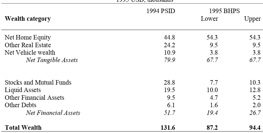
Table 1 lists mean values of wealth and its components for both countries. Total household wealth
is about a third higher in the US, but within asset category differences are far larger. Total non-financial
assets held by households are reasonably similar in the UK and US. Within that sub-aggregate, British
households actually have greater absolute and relative amounts of wealth in home equity than American
households do. Converted to a common currency, mean housing equity is almost ten thousand dollars
more than their American counterparts. Similarly, British households hold 62% of their total household
wealth as home equity: the comparable percent for American households is only 34%.
The other striking difference between UK and US lies instead in financial wealth where mean
values in America are more than twice those in Britain. These differences exist in all components of
financial wealth, but they are particularly large in stock market equity. On average, in the mid 1990s
American households owned about $20,000 more in corporate equity than their British counterparts.
Given the extreme skew in wealth distributions, means can be poor summary statistics for wealth.
In a previous paper (Banks, Blundell, and Smith (2000)), we have shown that total net wealth and financial
wealth distributions in both countries were extremely unequally distributed. Turning to differences
slightly higher among British households while median financial assets were somewhat greater among
American households. Rather the critical differences lie in the upper tails of the wealth distribution,
especially in financial assets. No matter which assumption about joint or separate ownership of assets is
made in the BHPS, the top fifth of American households have considerably more financial wealth than the
top fifth of British households do. The between country discrepancy in financial wealth expanded rapidly
as we move up the respective financial wealth distributions.
These wealth differences are not due to age and income differences between the countries. Banks,
Blundell and Smith (2000) demonstrate that, within age groups, net financial wealth in both countries
increases with household income albeit in a highly non-linear way and that at almost all points in the
age-income distribution US households are holding more financial wealth than their UK counterparts. The
same breakdown for net total wealth shows that for almost all of the younger age-income groups UK
households have at least as much wealth, if not slightly more, than their US counterparts.
3. A Comparison of Four Markets - Housing and Stock Markets in the US and the UK
To set a background for this paper, we first describe the most salient trends in housing and equity
markets in these two countries during the last few decades. Our description includes trends and differences
in rates of ownership, rates of return, and amounts of wealth held in these forms.
3.1 Rates of Asset Ownership: Housing
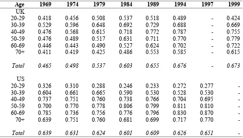
Table 2 lists the proportion of households who are homeowners, by the age of head of household,
for selected years in both countries. While aggregate rates of home ownership are now not that dissimilar
(around two-thirds in both countries in the most recent year listed), there are striking differences by age.3
Home ownership rates amongst young households are far higher in the UK than in the US, with
differences as big as twenty percentage points for householders between ages 20-29. While not as large,
2 Given that this is close to the OECD PPP conversion rates for this time (1.55 in 1994 and 1.53 in 1995) our
comparisons are unaffected by the use of exchange rate as opposed to PPP Conversion factors.
the fraction of households ages 30-39 is currently double digit larger in the UK. The offset to the greater
rates of home ownership among young British householders is the much lower historical rates among older
households in the UK. For example, among those over age 60, the prevalence of owning a home in 1984
was more than twenty percentage points larger in the US than in the UK.
Table 2 also suggests that there are stronger cyclic and trend effects on home ownership rates in
the UK compared to the US. Although the levels are always above their US counterparts, there was a sharp
upswing in home ownership among the youngest British household heads (those between ages 20-29)
which reached its peak between 1984 and 1988, during the height of a housing boom. Since that year, the
trend reversed and the proportion of homeowners amongst the youngest group in the UK fell. With lower
amplitude, a similar pattern exists among those aged 30-39. We return below to the question of why
cyclic variation in home ownership may be larger in the UK.
There are impressive cohort effects in UK home ownership with secular changes concentrated
among older households. For example, among British households ages 50-59, home ownership rates
increased by almost thirty percentage points after 1974. While not confined to that time period, the size of
the increase in home ownership is largest in the five-year interval between 1979 and 1984.
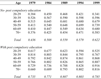
Table 3 presents the same data separately for UK households based on whether the head had some
post-compulsory education. This dramatic secular increase in home ownership in Britain is concentrated
among those with less education. Once again examining those ages 50-59, there was a 32 percentage point
increase in home ownership among those with no post-compulsory schooling compared to 12 percentage
point increase among those households whose head had moved beyond compulsory schooling levels.
The structure of these differences in home ownership between the UK and US raise several
questions. One question is what accounted for the magnitude and structure of the dramatic secular shift in
the UK. Given its timing, one contributing factor is the 'right-to-buy' scheme for public housing tenants,
which was introduced in 1980. Under this scheme those households who had been renting in government
local authorities. The house was valued at current market value but discounts, varying between 30% and
60%, were applied according to how long you had been living there.
The ‘right to buy’ program is consistent with the main features of the data in Tables 2 and 3. Most
important, public housing tenants are concentrated amongst the less educated where most of the increase
in home ownership occurred. Secondly, the concentration of change was among middle age and older
household who had longer tenure and could met the minimum tenure requirement and who also may have
accumulated a bit of savings for down payment.
The more difficult question arising from Table 2, and one on which we focus in this paper, is why
rates of home ownership are much higher among younger UK households. One possibility is the structure
of mortgages themselves. The typical UK model is characterized by a low down payment (5% to 10%),
variable interest rates and a fairly low take up of mortgage interest insurance. The typical US mortgage has
a higher down payment (20%), fixed interest rates4 and often is accompanied by mortgage interest
insurance, generating a more stable inter-temporal financial commitment (see Chiuri and Jappelli (2000)
for an institutional differences discussion). Differences in down payment requirements alone shortens the
time (compared to American households) it takes young British households to save in order to reach their
required down payments.5
Differences in housing wealth accumulation could be driven by other factors in the housing
market. Rental market rigidities or failures commonly thought to exist in the UK could be one issue.
Renters’ right rules are far more common in the UK, making it difficult to evict existing tenants. This may
explain differences in ownership rates among the young but not differences in the amount and growth of
net equity in housing held by homeowners. The low ownership rates among older British most likely lies
4 In the 1996 PSID sample, only 20.8% of households with mortgages had variable rate mortgages.
in a combination of the widespread availability of public housing to their generations as well as their much
lower levels of economic status compared to US households.
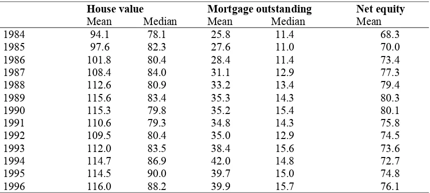
Table 4 provides another view of the housing market dynamics in the two countries by listing
yearly values of home values and outstanding mortgages for homeowners.6 The value of British homes is
always above that of their American counterparts. For example, in 1994 the median value of a home in the
UK is about 14% higher than the median home value in the US. Unless one has a strong prior that British
homes are in some sense ‘better’ than American homes, this price differential may simply indicate that
price of housing is higher in the UK. If so, the advantage of British households in housing wealth raises
some conceptual questions of whether this type of wealth advantage should be treated on a par with wealth
differences that emerge in other assets. If British homes are more expensive for the same quality and
demand is inelastic, British households will spend more on housing as discussed in section 4 below.
Table 4 also indicates that the higher net-equity held in British homes in part reflects higher
housing prices in the UK but also the smaller outstanding mortgages in the UK. This mortgage differential
prevails in spite of the fact that initial down payments requirements are lower in the UK than in the US.
This in turn suggests that compared to their US counterparts British households may not engage in
significant amounts of refinancing of their homes as real housing prices rise and capital gains are
accumulated. Consistent with this view, note the significant increase in outstanding mortgages in the
United States at a pace that parallels that of real housing prices so that net housing equity has remained
flat. While refinancing of homes has become reasonably commonplace in the United States over the last
decade or so (data from the 1996 PSID indicate that 37% of households with existing mortgages had
refinanced), this phenomenon appears to be much less important in the UK. British households seem to be
far more cautious in using wealth accumulated through capital gains in housing for other purposes.
3.2 Rates of Asset Ownership – Stock
Using the PSID, one-quarter of US households directly owned some stock in 1984, a fraction that
grows to 40% by 1999. Direct share ownership was far less common among British households especially
in the early 1980s. Figure 1 plots the time-series pattern of equity ownership in the UK between 1978 and
1996. By the mid 1980s, British household equity ownership rates had been stable and hovered just below
10%- well less US figure in 1984. Starting in 1984, equity ownership grew more rapidly in the UK than in
the US. While the gap in equity ownership has narrowed, by the mid 1990s almost one-quarter of British
households directly owned stock compared to one-third of American households.
Table 5 lists stock ownership rates by age in a form similar to that displayed in Table 4. Consistent
with Figure 1, secular changes in British stock ownership look much like classic calendar year effects.
There was almost no change between 1979 and 1984, followed by a sharp increase during the next five
years with very little change thereafter. These increases in stock ownership were slightly larger among
middle age households, but in general one is struck by the near uniformity in increases in prevalence
across all age groups. Not shown in Table 5, stock ownership expanded by a somewhat greater amount
among more educated British households.7
The same questions asked about home ownership are relevant to equity markets as well. Why the
inter-country differences and why the massive secular shifts in the UK? In the UK most of this increase
was concentrated in a four year period from 1985 to 1989, coinciding with the flotation of previously
nationalized public utilities such as British Telecom (1984) and British Gas (1986). Around this time, the
UK government introduced also a further set of measures aimed at promoting a ‘share-owning
democracy’ – namely tax-favored employee share ownership schemes. In the US the increase in share
ownership was more gradual throughout the 1980s no doubt induced by rising rates of return. One result of
these trends was that although the stock market boom was relatively similar across the countries, the
The differences between the two countries in stock ownership are again more difficult to answer.
One possible explanation is that market conditions, in particular transaction costs, taxes or information,
differ across the two countries. Certainly prior to the mid 1980’s in Britain there was a tax bias away from
direct holdings of equity towards wealth held in housing or occupational pensions, since equity was more
heavily taxed than consumption, and housing and pensions benefited from tax advantages relative to
consumption. Given the structure of the tax system these differences were significantly greater in times of
high inflation.8 However, the introduction of Personal Equity Plans and Employee Share Ownership
schemes meant that, from 1987 onwards equity could be held in a more favorably taxed manner by British
households. Indeed, Personal Equity Plans give holdings of equity an identical tax treatment to IRA’s or
401(k)’s, i.e. neutral with respect to consumption.9 These tax differences are discussed in section 4.
Another pertinent difference is stamp duty, where a 0.5% charge is levied on all share transactions
in the UK. But for infrequently traded portfolios such a difference is unlikely to be behind the marked
differences in share ownership observed across the two countries. Finally, there could be differences in the
information individuals have about stock market investment opportunities. Whilst this is a plausible
explanation for differences in the middle of the income distribution there are cross-country differences
even in the very highest percentiles of the income or wealth distribution, where such information
differences are unlikely to be so pronounced.
7 For example, between 1984 and 1989, stock ownership rates increased by eleven percentage points among those who stopped at the compulsory schooling level while it increased by 17 percentage points among household heads with more than a compulsory school education.
An alternative explanation for these differences, and possibly for higher accumulations of
financial wealth in America compared to most of Europe (including the UK) more generally, involves
differences in attitudes toward capitalist financial institutions (see Banks, Blundell, and Smith (2000)).
Especially during the 1970s and early 1980s, it is probably a fair characterization that there was more
distrust of the fairness of capitalism as an economic system at least among significant segments of the
European population. The stock market is one of most vivid capitalist symbols so this distrust may have
resulted in lower average participation in equity markets among Europeans. This could be one reason why
the equity boom that eventually occurred in the UK affected fewer households. However, the results
obtained by Banks, Blundell, and Smith (2000) suggests that only a part of the differences in equity
ownership can be explained by ideology differences between the countries.
If transaction costs, taxes, and ideology can not fully explain the low rates of stock ownership in
the UK, where do go from there? Below we provide a new explanation for these low rates of equity
ownership that are founded not in the institutional character of the equity markets in the two countries but
rather in differences in the two housing markets.
3.3 Rates of Return on Assets
Figure 2 plots inflation adjusted equity price indexes for both countries, each expressed relative to
a 1980 base10. The magnitude of the recent stock market boom in both countries is impressive even
compared to historical equity premiums. For example, real equity prices in the UK are about two and
one-half times larger in real terms in 1995 as they were in 1980- slightly larger than the equity appreciation in
the US over the same period. Yet, measured from this 1980 base, it is remarkable how similar equity
appreciation has been in both countries. US equity rates of return would be higher than those in the UK if
the mid 1970s was used instead as the reference suggesting that up to 1980 the (recent) historical
experience in the stock market was more favorable in America. Still, the compelling message from Figure
2 is that differential rates of return in each country’s equity markets during the 1980s and 1990s can not
explain the quite different levels of financial wealth holdings in each country by the mid 1990s.11
Similarly, Figure 3 shows real indices of average house prices for the US and UK over the period
1974 to 1998. As with the indices for equity returns, both series are normalized to unity in 1980.
Immediately apparent is the much larger volatility of housing prices in the UK, with real prices rising by
50% over the period 1980 to 1989 and then falling back to it’s previous value by 1992. Over the period as
a whole, however, real returns were similar across the two countries and much smaller than those realized
in the equity market. In addition, the highly volatile returns to housing equity and variable interest rates
leaves British households much exposed to business cycle vagaries. This should make them much more
cautious than Americans would be to refinancing their homes during housing price upswings and
converting the funds into financial assets. 12
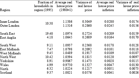
The UK index also hides considerable differences across regions with some being much more
volatile than others. In Table 6 we present summary statistics for house prices from the regional sub
indices, showing both average house prices and average house price inflation over the period as a whole,
along with the corresponding variances. Immediately clear is that London and the South East of England,
in which almost 30% of UK households are located) face considerably higher volatility than the average
UK index. We return to this below.
3.4 Differences in wealth holdings in housing and stock
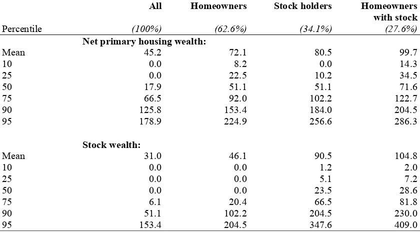
In Tables 7a and 7b we report percentiles of net primary housing wealth and stock wealth, in both
the US and the UK, by home ownership and stock ownership status. Note that in this table and those that
11 For simplicity, our comparison relates to stock prices as opposed to stock returns, but dividend yields are comparable or, if anything, higher in the UK so this cannot account for higher US stock holdings (see Bond, Chennels and Devereux (1998), for example).
12 To this point we have discussed income, housing price and stock price risk in isolation. In deciding on the composition of their wealth portfolios, households will also consider the correlation of these risks. This is a
follow, we use the upper bound of household stock wealth in the UK. Since the UK has less stock wealth,
if anything, differences between the US and the UK will be underestimated. For all types of households
the distribution of wealth held in the form of primary housing is higher at each point in the UK than in the
US, although the differences are largest in the bottom three-quarters of the distribution.
In contrast, stock holdings are much higher among American households. In the mid 1990s, the
mean value of shares in America was three times as large as in Britain and was about twice as large when
considering shareholders only. In both countries, distributions of stock values are highly skewed, with
extreme concentrations in five to ten percent of households. But at all points in the distributions, the value
of American holdings are multiples of two or three of those held by British households. 13
The conditional distributions contained in Table 7 hint at a greater separation of stock and housing
holdings among British households. Among stockholders, the mean value of stock holdings in the UK is
only three thousand dollars higher if British households are also homeowners. The ‘effect’ of home
ownership on stock wealth is much higher in the US especially among large stock values.
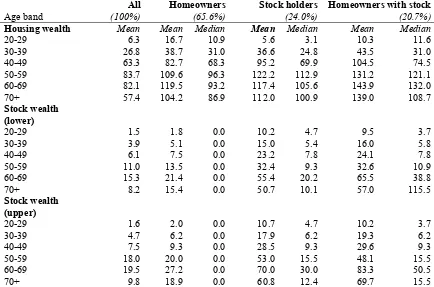
Tables 8a and 8b present means and medians of stock and housing wealth by age band in the two
countries, split according to whether households have stocks, housing wealth or both. Looking at the
patterns by age a striking difference emerges. Homeowners in the UK demonstrate a substantial age
gradient in their housing wealth, at both the mean and median. Median net housing wealth for the 40-49
year olds is seven times higher than that for the 20-29 year old. This gradient is much flatter in the US,
with the corresponding ratio being just over three. The reverse is true for stock wealth – the age gradient of
stock wealth for stock owners in the UK is extremely shallow,14 whereas in the US stock wealth rises by a
exists between housing price risk and GDP risk. Moreover, this correlation is significantly higher in the UK than in the US consistent with our view that housing supply elasticity is much smaller in the UK
13 Banks, Blundell and Smith (2000) show that the comparison between the 1995 BHPS and the 1984 PSID reveals that, both for the full population of households and for shareholders only, the distribution of share values held by households are virtually identical. That is, after the stock market surge in both countries, British households had stock wealth similar to American households ten years earlier. In the early 1980s, however, we know that in light of the subsequent extremely large increase in share ownership British households’ stock holdings were considerably smaller than their American counterparts. This initial condition difference between the two countries would have profound impacts on wealth distributions by the mid 1990s.
factor of almost ten for stock holders aged 50 in comparison to those aged 20-29. Looking at just those
who own both homes and stocks the differences still emerge. It is these differences which we will explore
in more detail later in the paper, and which motivates the design of our modeling exercise.
4. A Model of Housing Tenure Choice and Portfolio Decisions
4.1 The demand for housing services
In the simplest model housing demand is purely a function of family size. It will therefore increase
over the early period of the adult lifecycle as family size increases. In Figure 4, we present profiles for
house size, with each line representing a thirty year time series of the average number of rooms for a
year-of-birth cohort over the time period 1968-1998. The Figure shows that, in the UK, there is a strong
increase in size of house, as measured by the number of rooms, as the head of household grows older,
flattening out around the age 40 but rising steeply from the 20s to the 30s. For this reason we can frame
our discussion in terms of a stylized model with three stages in an early adult life-cycle: leaving home,
living as a couple but without children, living as a couple with children. There is also little evidence of
strong cohort effects during the early part of the adult lifecycle, as evidenced by the lack of vertical
differences between each cohorts profiles up to age 40. Hence this rise is the same whether we look at
individual date of birth cohorts, as in the figure, or pool across cohorts.
In general housing demand will also depend on the unit price of services, the level of (expected)
wealth and the degree of uncertainty over all these variables. It is likely that demand for housing services
is price inelastic. Consequently expenditure on housing services will be increasing in the price of housing
services. According to our numbers, the median value of a US owned home in 1994 is about 14% less than
the median price (value) of an UK owned home. Unless we think that there is 14% more utility involved,
this is evidence of a higher unit price in the UK. A higher unit price in the UK will induce a higher level of
4.2. The choice of housing tenure
At the start of the adult lifecycle, housing tenure decisions occur in two stages. First, a choice of
when to leave the parental home and then whether to rent or to buy. Strictly speaking, the latter is not a
portfolio decision since, if a house is bought and continuously re-mortgaged, there is no necessity to hold
any housing equity. Yet, ownership is a prerequisite for securing housing equity and so the decision to
own may be influenced by portfolio choices as well as pure service flow considerations. A house may also
be owned without any desire to accumulate housing equity simply because it is an efficient way to achieve
a desired flow of housing services. For a household with little expected mobility and heterogeneity of
tastes, owning can be the least cost way of achieving a desired level of housing service.
Young households who first decide to rent remain potential purchasers of a starter home as soon
as they are able to secure a down payment. In the decision to leave the parental home, credit constraints
will also play an important role as such constraints are typically binding on young adults who must
accumulate sufficient wealth to meet down payment and collateral requirements. Consequently, the
income of the young will be important and the volatility of incomes of young people rather, than in per
capita income per se, will be critical in generating swings in housing transactions.15 Higher down
payments lengthen the time required to build up enough wealth to satisfy lenders and will make first time
homebuyers older on average. Similarly, inadequate rental markets may delay the age at which one leaves
the parental home but lower the age at which one buys the first home. This last point is explored, using the
BHPS data used in our analysis, in Ermisch (1999) who finds empirical support for the economic
conditions of the housing market relating to the household formation choices of the young in Britain.
In light of the data in Figure 4, and of empirical and theoretical models of housing market
dynamics (see Di Salvo and Ermisch (1997) and Ortalo-Magne and Rady (1998) respectively, for
example) the initial home purchase is best seen as the first step in a property ladder. If there is some job or
demographic mobility expected then, because of lower transaction costs, the rental market may provide a
lower cost way of choosing an optimal path for housing services. If house prices are variable the rental
market may also provide a contract insuring against some of that risk. But by leaving equity in their home,
first time homeowners are partially self-insuring against price fluctuations in the housing market. While a
price increase will raise the price (and required down payment) on the second home, the price of the first
home is also increasing providing additional resources for that now larger down payment. A symmetric
argument obtains during periods of housing price declines.
As incomes and family sizes grow, these now slightly older young adults hope to buy a larger,
more expensive home. The time interval between these purchases is once again governed by the length of
time it takes to secure the larger down payment needed on the bigger house. Low down payment
requirements will shorten the interval between home purchases. In addition, any capital gains on the first
house may be used to help buy the second. Capital gains during boom will tend to shorten the time interval
between first and second home purchase while capital losses during downturns will lengthen this interval.
4.3 House Price Uncertainty and the Choice between Stock and Housing Equity
Each household has a desired level of total wealth. This level will depend on expected future
income and consumption streams as well as the returns on assets. First consider the portfolio demand for
housing equity. If house prices are variable and uncertain then, given the increased demand over the early
part of the lifecycle, housing equity will be an important source of insurance against house price risk. The
larger the uncertainty in house prices and the steeper the demand over the life-cycle, the more important is
the insurance aspect of housing equity.
Conditional on being an owner, therefore, the higher the level of house price uncertainty the larger
the demand to pay down the mortgage and to hold wealth in housing equity. This will be particularly the
case for households early in their lifecycle as they anticipate stepping up the property ladder. It would
make little sense for risk adverse young households who face housing price volatility to invest their assets
in the stock market even if stock price and housing price risks are uncorrelated.
The tax treatment of mortgage repayments will also influence the level of mortgage held and the
consume more housing services and to use ownership as a vehicle for that consumption but not necessarily
to pay down the mortgage. Rather it might be optimal to invest in another risky asset rather than pay down
the outstanding mortgage or even to re-mortgage a housing equity capital gain.
4.4 The Supply of Housing Services
There are two aspects the supply of housing services which are central to our model. First, a more
inelastic supply will induce a larger sensitivity of house prices to fluctuations in demand, in particular to
fluctuations in the income of young first time buyers. The second aspect relates to the rental market.
Imperfections and/or regulation of the private rental market may make it difficult for the young to use
rental housing as the step between leaving the parental home and acquiring a house. The rental market
may also be dominated by the public sector in which case the allocation mechanism may be less sensitive
to the demand of young households.
A consequence of inelastic demand is that expenditure on housing services will be increasing in
the price of housing services. According to our numbers, the median value of a US owned home in 1994 is
about 14% less than the median price (value) of an UK owned home. Unless we think that there is 14%
more utility involved, this is evidence of a higher unit price in the UK. A higher unit price in the UK will
induce a higher level of expenditure conditional on all the other factors.
4.5 Model Predictions
The model predictions for the UK relative to the US as households move through their early
life-cycle profile is clear. The demand for housing services will increase as family size increases. Consider the
three stages of our stylized life-cycle profile: leaving home, living independently without children, living
with children. The model predicts that the level of owner occupation at the second stage should be lower in
the US relative to the UK if the deposit and mobility motivations dominate the tax advantage. This is
reinforced by the higher house price volatility in the UK which makes owner occupation more likely for
This prediction could also be rationalized by an inefficient rental market in the UK. However, the
arguments also suggest that the UK would have a higher level of housing equity for volatility reasons but
that this would be reduced once full household size is reached at stage three in the early life-cycle profile
since the positive volatility effect would disappear. Other things equal the tax advantage in the US would
make households more likely to be owners in the US and less likely to pay down capital – and less likely
accumulate housing equity.
The higher volatility in the UK increases the desire to hold housing equity in the UK for those
households in the second stage of their demographic profile, i.e. those who expect to increase there family
size. In turn this increases the desire to be an owner for such households in the UK. We expect more
owners and a higher paying down of outstanding housing debt in the UK, a higher level of housing equity
in the UK. The later but not the former of these is predicted by the tax advantage.
5. The Housing Market and Income Risk of the Young
5.1 The Housing Market
Our model on housing markets places great weight on the role of young households and on the
role of housing and stock in portfolios over the life-cycle. To evaluate whether the young merit such an
emphasis, we examine individuals who purchased a new home between waves of the PSID and BHPS
samples. Across all ages, about one in twenty household heads in both countries are observed to have
bought a new home since the previous wave of the panel. It is also clear that young people were far more
active in the housing market. For example, 12% of British household heads between the ages of 20-29 had
bought a new home during the last year. The comparable number in the US was 9%.
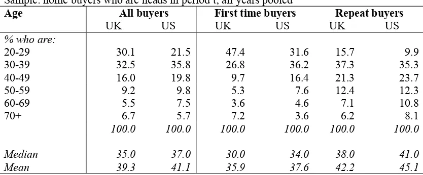
Table 9 lists the age distribution of household heads who purchased a home between the annual
waves of each survey.16 Besides describing all homebuyers, this data are stratified by whether household
heads were ‘first time’ buyers or ‘repeat’ buyers. Repeat buyers represent those who had lived in a home
that they owned before this new purchase while ‘first time’ buyers were not living in a home that they had
personally owned right before this new purchase.17
Consistent with our view that they constitute the active part of the housing market, new
homebuyers are much younger than the average homeowner is.18 Moreover, the typical purchaser of a
new home is a good deal younger in the UK than in the US. For example, 63% of all new buyers in the UK
are less than forty years old with a median age of 35. The comparable numbers for the US are 57% and a
median age of 37. The differences between the two countries are most striking among those household
heads between ages 20 and 29, who constitute 30% of all new UK buyers compared to 22% in the US.
‘First time’ buyers are especially young with median ages of only 30 (UK) and 34 (US).
Household heads less than thirty years old comprise almost half (47%) of all first time buyers in Britain,
much higher than the comparable US proportion of about a third (32%). Not surprisingly, ‘repeat’ buyers
are somewhat older in both countries, but even here the median ages are only 38 (UK) and 41 (US). More
than half of repeat homebuyers in the UK are less than forty years old.
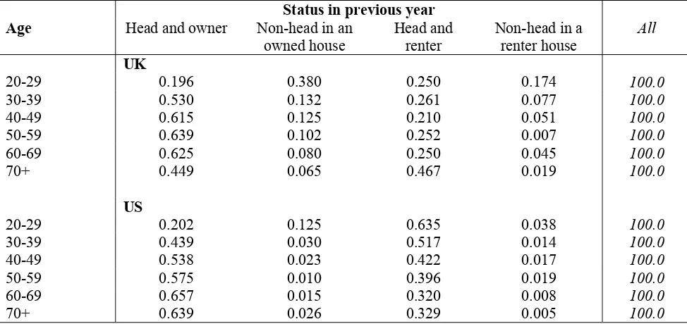
Age is one dimension in which new homebuyers differ in the two countries.19 Table 10 tries to
illuminate an additional dimension by listing prevalence rates of new owners by their joint ownership and
headship status in the previous survey wave. A similar fraction of new buyers in both countries had
owned their own home in the prior wave. The principal difference emerges in the third column where
there exists a far greater fraction of American households who made a transition from renting a place of
their own to buying one. These inter-country differences are especially large among young people (aged
20-29). In particular, 64% of new buyers in this age group in the US were previously household heads
who were renters. The comparable British figure is only one quarter. The counterweight is the large
17 More precisely, ‘first time’ buyers consist of those who lived in a rental house in the previous survey wave and those who lived in a owned home with their parents or
18 For example, in 1994 the mean age of all homeowners was 50.4 in the UK and 51.3 in the US.
19 As documented in section 3, over recent years the relative tax status of housing and stock wealth has been
fraction of young homebuyers in Britain who were not heads of household in the prior year (55% in the
UK compared to 16% in the US). These young British non-household heads were more than twice as
likely to live in an owned as opposed to a rented home- it was simply not a home that they owned.
Among those who had lived previously in an owned home, the dominant situation for those
between ages 20-29 was that they depart the parental home. While this is true for both countries, this is a
far larger group of young people in the UK than it is in the US. A key difference between the two
countries concerns what happens when a young person first leaves the parental home. Across the years we
examined, about one-fifth of British adults 20-29 who were living in the parental home moved out the next
year. The US number is only slightly larger (about one-fourth). While the likelihood of leaving the
parental home was roughly similar, where these British and American young adults went could not have
been more different. Table 11 indicates that almost half of all young adults aged 20-29 in Britain who left
the parental nest bought their own home. In sharp contrast, this fraction is only 18% in the United States.
While much smaller numbers are making this transition among those ages 30-39, the differences in the
type of transition between the two countries remains. 20
The data in this section documented the following important differences between new homebuyers
in the UK and the US. New homebuyers are disproportionately very young adults with a particularly
pronounced tilt toward the young in Britain. When they leave their parents’ home, Americans first tend to
live in rental housing either on their own or with their spouse or partner. No doubt due to difficulties in
the British rental market, when they leave their parents British youth tend to skip over this intermediate
step and go immediately on to purchasing their own house. Finally, these trends have interacted with
massive compositional changes in household population so that increasing fractions of young homeowners
are not currently married.
5.2 Income Risk
Our emphasis on the young also points to a potentially important role for income risk in this
model. There are two aspects of income 'risk' that will be useful to distinguish. The first is the systematic
variation in aggregate first-time buyer income or shocks to income. As we noted above it is this that
generates variation in the demand for first-time purchases. The second possible measure of income
variance is the level of within period income risk for each age group. We focus on the former since the
latter will act as background risk and will only indirectly effects the demand curve through risk aversion.
A higher level of the first will create fluctuations in the price of housing provided supply is inelastic.
To investigate this we need to examine whether the variation of the age specific aggregate shocks
is larger for the young. The framework we adopt follows Banks, Blundell and Brugiavini (2000) and
separates aggregate from idiosyncratic risk. To estimate the aggregate variance for each age band, we
regress average log income for each cohort on its lagged value for the same cohort and a list of changes in
observable demographic characteristics. We then compute the variance of the time and cohort specific
income shocks from this regression for each age group. The results of this regression using the repeated
cross sections from the UK FES (1978-1999) are presented in Table 11.
In a simple liquidity constrained model, the variance of income itself rather than the variance of
income shocks would determine fluctuations in demand. A comparison of the two measures of the
aggregate variance for broad age bands in the UK is presented in the first two columns of Table 11. For
both measures there is a steep decline in aggregate income variation for as we move from households
whose heads are in their 20s to those households where the head is in the 30s age band.
Note that the level of income variation rises systematically over time, especially in the 1980s. So
that our measure of risk for the young may be an underestimate since the young will presumably also face
more risk as a result of uncertainty about future demographics and household formation.
6. How Well Does the Model Explain the Data?
The model developed in section 4 was motivated by a number of facts relating to housing tenure
choice, to housing equity and to the stock of wealth holdings by households over their life-cycle in the UK
and the US. In this section we ask whether the model can provide a convincing explanation and whether it
can do better than other competing explanations.
6.1 Implications of the Model
The principal implications of our model stem from the significantly higher volatility of house
prices in the UK. This starting point is fundamental and we have two underlying explanations for it. First,
the supply of housing is likely to be more inelastic in the UK in part due to the greater population density
there. This is most clearly seen in the dominance of the greater London area in the British housing market.
Around 30% of all homes in England are located within the Southeast (including Greater London). Not
only is the available space limited there, but new housing construction or conversion is heavily regulated
and costly to build. This more inelastic supply implies that for any given demand side fluctuations,
housing prices will be more volatile in the UK than in the US.
Second, house prices are more sensitive to the variation in first time buyer demand and therefore
the volatility of first time buyer incomes. Because British new home buyers are younger and therefore
positioned on the more volatile part of the income risk-age curve, income fluctuations inducing demand
side swings will also contribute to the greater price volatility in the British housing market.
In addition to more volatile prices, down-payment requirements are less onerous in the UK and the
rental market is less efficient. In our model, these conditions all conspire to lead young UK households to
move into owner occupation rather than to rent and to do this at an earlier age. This pattern of home
ownership is born out by the data. We find a significantly lower use of the rental market in the UK among
occupation. Of those adults aged 20-29 observed to leave the parental home in the BHPS 46.6% became
owner-occupiers directly, as opposed to only 15.0% for their PSID counterparts. Although the group is
much smaller, similar differences pertain for the 30-39 age group.
Our model also had implications for portfolio choice. The higher house price volatility in the UK
makes it optimal for those young households who expect to move up the property ladder to hold housing
equity. Young homeowners in the UK, who plan to upgrade their housing by purchasing a larger, newer
home as their incomes and families expand, may face considerable housing price risk. One method of
self-insuring against housing price volatility would be to maintain a large fraction of household wealth in
housing equity thereby matching possible variation in the value of one’s current home with the price of
any desired home upgrade.21 In contrast, a quite risky strategy among young homeowners would be to
hold much of their wealth in stock. Even if housing price and stock price risks are uncorrelated, a
downturn in the equity market could make it quite difficult for young homeowners (who have limited
amounts of household wealth) to reach their down payment goals for the new home.
For young UK households facing higher house price risk and lower down-payment requirements,
the model predicts that they enter the housing owning market earlier, cover a very large percentage of the
house price by mortgage and then pay down the mortgage as a saving instrument for future movements up
the property ladder. Early in their adult lifecycle we would expect to see a higher proportion of young
owner-occupier households in the UK. At this point they would have little equity in housing and hold
relatively large mortgages. But as they move through the early part of their adult lifecycle they would
rather accumulate housing equity than stock. Consequently, we predict that compared to the US, in the UK
age gradients in housing equity will be steeper and in stock equity less in the early part of the lifecycle.
From Figure 4 we might expect this comparison to be particularly strong in the 20s and 30s and then to
dampen out in the 40s and 50s as the property ladder reaches a plateau.
The housing and stock wealth numbers reported in Table 8 would appear to be most relevant for
testing these predictions. Table 8 shows, as predicted, that UK households indeed have a much steeper
gradient in the accumulation of wealth in housing equity. The strong gradient for UK households is
evident in both the mean and the median of housing wealth in the first panel of Table 8a. The model also
implies that the gradient should be even steeper among homeowners, especially those facing high housing
price risk. Mean housing wealth rising by a factor of two between 20s and 30s and then again by the same
factor between 30s and 40s for homeowners in the UK. The reverse is true for stock wealth. Compared to
the US, the UK shows little gradient in stock wealth for those households early in their adult life cycle. For
stock, due to a few large outliers the median is probably a more robust measure, but even for the median
there is little evidence of a gradient in the UK. In the US the gradient in stock wealth is even more striking
than it was for housing wealth in the UK.
6.2 Biases in age gradients for the portfolios of the young
There are potential problems with our reliance on the data in Table 8. First, cohort effects that we
have seen are quite real in housing and equity markets may confound them. Second, they describe the
pattern of wealth holdings by age of household heads and many young adults are in households headed by
their parents and thus appear in households with older heads.
Cohort Effects
The data in Table 8 are cross-sectional age profiles and may be contaminated by year and cohort
effects. If cohort and time effects are the same across the two countries, our comparisons of age profiles
may be less affected by this issue than for each individual country age profile. Yet the evidence in Tables
2 and 5 – listing ownership age profiles by country and year – suggests this may not be the case.
There are two types of cohort-year effects that may well affect our comparisons. The first are
unique events that differentially affected the incentives to own homes or stocks in the two countries. The
We first examine the impact of capital gains. For stocks, average rate of returns have been high
and approximately the same in both countries but there remains a possibility that middle aged American
cohorts benefited by being differentially exposed to the stock market (in comparison to the UK) in the
mid-eighties. Fortunately, because questions are included on new stock purchases and sales we are able in
the US data to separate out that part of wealth accumulation in stock that is due to capital gains. To
examine the impact of capital gains, we list in the first column of Table 13 the cross sectional holdings of
stock wealth by age in the US in 1984. The next column labeled realized shows the actual stock wealth of
these 1984 age groups ten years later. The large within cohort increases in stock wealth are certainly
suggestive of significant capital gains in stocks. While these adjusted profiles indicate a much less steep
pure lifecycle increase in stock wealth, even the capital gains adjusted data for the US exhibit a larger age
gradient than the unadjusted UK age gradient. Since the British stock age gradient is also exaggerated by
capital gains, we conclude that the steeper US age gradient for stock wealth is not solely a consequence of
capital gains in stocks. For housing, however, the time series of returns suggests that over the period as a
whole (particularly to 1994) returns were similar in both countries but more volatile in the UK.
In addition to the impact of differential capital gains, there are other cohort-year effects that
differentially impact both stock and housing markets in the UK. However, these year effects are specific
to a very narrow time period allowing us to control for their impact. For example, the large increase in
stock ownership rates in the UK due to the flotation of national industries was concentrated during the
time period 1984-1989. By limiting our comparisons to the post 1989 period, we can minimize the
impact of this effect. We do so in Table 14 by listing in the first column 1989 age profiles of stock
ownership in both countries. In the adjacent column are listed the ownership rates of these age groups ten
years later. In all cases, there was a much more rapid buildup in stock ownership in the US compared to
the UK.
Household Composition
So far we have been considering age profiles of housing and stock wealth computed by the age
and in the case of joint ownership, the oldest of the joint owners. Given the higher frequency of young
adults living in households with older heads in the UK, Table 8 could display serious differential bias in
the age pattern of housing and stock holdings of the UK relative to the US. These biases apply to a
considerably wider set of problems and relationships of interest than this one alone.
There are two potential biases due to household composition in looking at differences in life-cycle
age profiles across countries. The very notion of a household (defined by the age of the head) results in
the consideration of a selected sample. In both countries there will be young adults, at the beginning of
their life-cycles, who are still in the parental home, or who in other non-spousal living arrangements, many
of whom will not be picked up in our calculations in the appropriate age band. To the extent that this group
is differentially sized in the two countries the age-profiles will be differentially affected.
Table 15 examines this issue by considering all adults in each age band (as opposed to just
household heads) and looking at the distribution of relationships to the head of the household in which
they live. Roughly one quarter of adults aged 20-29 in each country are still living with their parents (i.e.
they are children of the head). But this is where the similarities end. A higher proportion of young adults in
the UK are married or cohabiting with the household head, considerably less adults in the UK are actually
household heads, and considerably more are in ‘other’ arrangements, where amongst the young this group
is predominantly non-relatives.
This means that the country specific age-profiles may well be influenced by the fact that when
working at the household level we do not count many young individuals at the start of their life cycles.
These children of household heads will crop up instead in our tables as members of the households aged
40-49 or 50-59. These omitted young adults from the early age bands will tend to have lower housing (in
fact zero) and stock wealth so that age gradients will tend to be understated.
Table 15 indicates a second bias — there are substantially more single heads of household
amongst the young in the US than in the UK. Individuals in single and married households are treated
household are summed and treated as one. 22 When there are many young married households, average
assets are inflated and the age gradient of wealth is affected.23
The magnitude of the impacts of these biases on age profiles for wealth will depend, to some
extent on the amounts of wealth held by each group identified in Table 15. The discussion above makes it
clear that there is some reason to believe that even if there were no underlying differences in wealth
between young heads and other young adults we would still observe an unduly flat age profile. In fact the
situation is exacerbated because young heads (particularly when coupled with their spouses) typically have
more assets than their peers. Taking data at the individual level once more from the BHPS, the rate of
stock ownership amongst young (20-29) heads and spouses is 14.7%, compared with 8.6% for young
adults living in the parental home. Correspondingly, asset stocks are around 33% higher for this group also
(‘upper’ estimates are $4,034 for heads, $3,120 for children of heads and $612 for non-relatives; ‘lower’
estimates are $2,496, $1,160 and $545 respectively).
Using the UK data, in which asset values are actually collected from individual household
members, we can begin to understand the importance of such biases on our age wealth profiles.24 In Table
16 we recomputed age profiles for stock in the UK on a tax unit and an individual basis, as opposed to a
household basis. For the tax unit we define as separate units, all adults except spouses as opposed to just
looking at all households. Spouses’ assets are added to those of the head and the combined unit is counted
only once. For the individual analysis, we divide the assets in a married household by two and count each
adult in an age band as a distinct unit.
The final two columns of Table 16 repeat the household level medians from Table 8. The
differences in age profiles across different types of unit are not trivial. In particular, stock wealth is
22Individuals in married households may also individually accumulate more wealth due to marriage selection effects (being more prudent) or if marriage encourages savings.
23A further issue is that the way in which the BHPS data is collected, with asset stocks asked individually and then
questions about joint ownership following, one might expect this to impact on the difference between our ‘upper’ and ‘lower’ bounds for the youngest age group in particular. We use the upper bounds in Table 14.
differentially lower for the youngest tax units so that the resulting tax unit and individual age gradients are
much steeper than household unit gradients. For example, if at a household unit in the UK, the ratio of
median stock wealth of the 60-69-age band is 6.4 times that of the 20-29 age band. The comparable UK
number at the tax unit or individual unit level is about 10.6. These ratios are sufficiently different to raise
serious questions about the sensitivity of tests of the life-cycle model to the widespread use of household
unit analysis. However, no matter which UK unit of analysis is used the stock age gradients are always
much less than the household unit in the US where the comparable ratio of these two age groups is 17.
The US number itself would be much higher at the tax or individual unit level. Thus, we conclude that
while household composition is an extremely important issue, the biases it creates do not substantively
affect our conclusion that age gradients of housing equity are steeper in the UK while age gradients of
stocks are steeper in the US.
6.3 Other potential explanations
This combination of differences in ownership and the gradient of stock versus housing equity
between the UK and US gives support to our proposed model. However, it may well be that there are
many other explanations of the same phenomena that could perform equally well. We now turn to these.
The first, and most obvious potential candidate for these differences between the UK and the US is the tax
differentials, i.e. the possibility that the preferential treatment of mortgage debt in the US could drive all
the observed differences in net housing wealth. It is certainly true that tax differences can explain why
homeowners in the US maintain a relatively large mortgage debt. However, such a difference in tax
advantages will also make ownership more attractive over renting thus making it difficult to explain the
high demand for home ownership in the UK, relative to the US, among young households.
A second possibility is that rental market inefficiencies alone could drive the observed differences.
In this case, rental market inefficiencies could explain the lower use of the rental sector among younger
households in the UK. However, such an explanation taken on its own cannot explain why, once an owner,