A Review on Image Segmentation Clustering Algorithms

A Review on Image Segmentation Clustering

Algorithms

Devarshi Naik ,

Pinal Shah

Department of Information Technology, Charusat University CSPIT, Changa, di.Anand, GJ,India

Abstract— Clustering attempts to discover the set of

consequential groups where those within each group are more closely related to one another than the others assigned to different groups. Image segmentation is one of the most important precursors for image processing–based applications and has a crucial impact on the overall performance of the developed systems. Robust segmentation has been the subject of research for many years, but till now published work indicates that most of the developed image segmentation algorithms have been designed in conjunction with particular applications. The aim of the segmentation process consists of dividing the input image into several disjoint regions with similar characteristics such as colour and texture.

Keywords— Clustering, K-means, Fuzzy C-means, Expectation

Maximization, Self organizing map, Hierarchical, Graph Theoretic approach.

I. INTRODUCTION

Images are considered as one of the most important medium of conveying information. The main idea of the image segmentation is to group pixels in homogeneous regions and the usual approach to do this is by ‘common feature. Features can be represented by the space of colour, texture and gray levels, each exploring similarities between pixels of a region. The result of image segmentation is a set of regions that collectively cover the entire image, or a set of contours extracted from the image.

Robust image segmentation is a difficult task since often the scene objects are defined by image regions with non-homogenous texture and colour characteristics and in order to divide the input image into semantically meaningful regions many developed algorithms either use a priori knowledge in regard to the scene objects or employ the parameter estimation for local texture [1].

Clustering is the search for distinct groups in the feature space. It is expected that these groups have different structures and that can be clearly differentiated. The clustering task separates the data into number of partitions, which are volumes in the n-dimensional feature space. 

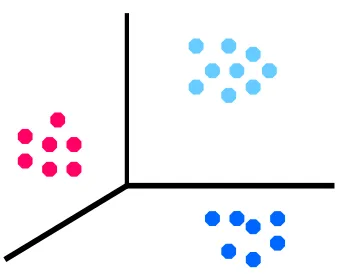
Clustering is a classification technique. Given a vector of N measurements describing each pixel or group of pixels (i.e., region) in an image, a similarity of the measurement vectors and therefore their clustering in the N-dimensional measurement space implies similarity of the corresponding pixels or pixel groups. Therefore, clustering in measurement space may be an indicator of similarity of image regions, and may be used for segmentation purposes.

Fig. 1 Similar data points grouped together into clusters

II. SEGMENTATION ALGORITHMS

Image segmentation is the first step in image analysis and pattern recognition. It is a critical and essential component of image analysis system, is one of the most difficult tasks in image processing, and determines the quality of the final result of analysis. Image segmentation is the process of dividing an image into different regions such that each region is homogeneous.

A. K-means Clustering

K-Means algorithm is an unsupervised clustering algorithm that classifies the input data points into multiple classes based on their inherent distance from each other.[3]

One of the most common iterative algorithms is the K-means algorithm [2], broadly used for its simplicity of implementation and convergence speed. K-means also produces relatively high quality clusters considering the low level of computation required. The k-means method aims to minimize the sum of squared distances between all points and the cluster centre. K-means algorithm is statistical clustering algorithm.

Data clustering is method that creates groups of objects (clusters). K-means algorithm is based upon the index of similarity or dissimilarity between pairs of data components. K-means algorithm is iterative, numerical, non-deterministic and unsupervised method[4]. K-means perform well with many data sets, but its good performance is limited mainly to compact groups.

generating globular clusters. The K-Means method is numerical, unsupervised, non deterministic and iterative.

Fig. 2 K-means clustering Process

(1)

The procedure follows a simple and easy way to classify a given data set through a certain number of clusters (assume k clusters) fixed a priori. The main idea is to define k centroids, one for each cluster. These centroids should be placed in a cunning way because of different location causes different result. So, the better choice is to place them as much as possible far away from each other [4]. The next step is to take each point belonging to a given data set and associate it to the nearest centroid. When no point is pending, the first step is completed and an early group age is done. At this point it is necessary to re-calculate k new centroids as bar centers of the clusters resulting from the previous step. After obtaining these k new centroids, a new binding has to be done between the same data set points and the nearest new centroid. A loop has been generated. As a result of this loop, one may notice that the k centroids change their location step by step until no more changes are done. In other words centroids do not move any more. Finally, this algorithm aims at minimizing an objective function, in this case a squared error function [4].

K-means algorithm has three basic disadvantages [4]:  K, the number of clusters must be determined.

 Different initial conditions produce different results.  The data far away from center pull the centers away

from optimum location.

The entire document should be in Times New Roman or Times font. Type 3 fonts must not be used. Other font types may be used if needed for special purposes.

B. Fuzzy c-means

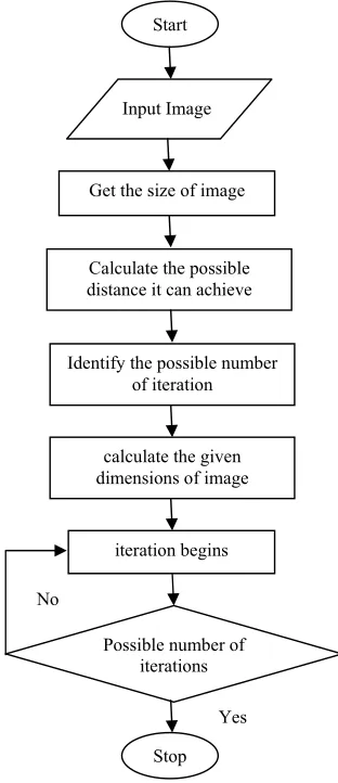
Fuzzy C-Mean (FCM) is an unsupervised clustering algorithm that has been applied to wide range of problems involving feature analysis, clustering and classifier design. FCM has a wide domain of applications such as agricultural engineering, astronomy, chemistry, geology, image analysis, medical diagnosis, shape analysis, and target recognition. With the developing of the fuzzy theory, the fuzzy c-means clustering algorithm based on Ruspini fuzzy clustering theory was proposed in 1980s[11].

Fig. 3 Fuzzy c-means clustering Process

An image can be represented in various feature spaces, and the FCM algorithm classifies the image by grouping similar data points in the feature space into clusters. This clustering is achieved by iteratively minimizing a cost function that is dependent on the distance of the pixels to the cluster centers in the feature domain. The pixels on an image are highly correlated, i.e. the pixels in the immediate neighbourhood possess nearly the same feature data. Therefore, the spatial relationship of neighbouring pixels is an important characteristic that can be of great aid in imaging segmentation.

The FCM algorithm assigns pixels to each category by using fuzzy memberships. Let X=(x1, x2,.,xN) denotes an image with N pixels to be partitioned into c clusters, where

Start

Input Image

Get the size of image

Calculate the possible distance it can achieve

Identify the possible number of iteration

calculate the given dimensions of image

iteration begins

Possible number of iterations

Stop No

xi represents multispectral (features) data. The algorithm is an iterative optimization that minimizes the cost function defined as follows:

(2) where uij represents the membership of pixel in the cluster, is the cluster center, is a norm metric, and m is a constant. The parameter m controls the fuzziness of the resulting partition, and m=2 is used in this study. The cost function is minimized when pixels close to the centroid of their clusters are assigned high membership values, and low membership values are assigned to pixels with data far from the centroid. The membership function represents the probability that a pixel belongs to a specific cluster.

C. Expectation Maximization

Expectation Maximization(EM) is one of the most common algorithms used for density estimation of data points in an unsupervised clustering. The algorithm relies on finding the maximum likelihood estimates of parameters when the data model depends on certain latent variables. In EM, alternating steps of Expectation (E) and Maximization (M) are performed iteratively till the results converge.

The E step computes an expectation of the likelihood by including the latent variables as if they were observed, and a maximization (M) step, which computes the maximum likelihood estimates of the parameters by maximizing the expected likelihood found on the last E step[3].

The parameters found on the M step are then used to begin another E step, and the process is repeated until convergence[3]. Expectation maximization clustering [12] estimates the probability densities of the classes using the Expectation Maximization (EM) algorithm. The result is an estimated set of K multivariate distributions each defining a cluster, with each sample vector assigned to the cluster with maximum conditional probability. Different assumptions on the model correspond to different constraints on the covariance matrices of each distribution. The less strict the constraints the more flexible the model, but at the same time more samples would be necessary for good estimates of the additional parameters. As always, the user of the algorithm is responsible for deciding the level of constraints to apply based on the amount of data available.

The expectation maximization algorithm is iterative statistical technique for maximizing complex probability that pixel belongs to segment [4]. The EM algorithm consists of 2 basic steps. In the first step is estimating the probability distribution of the variable and in the second step is increasing the log likelihood function. This iteration process repeats two steps and continuous until convergence at local optimum [4].

D. Hierarchical

Hierarchical clustering [2] creates a hierarchical tree of similarities between the vectors, called a dendrogram. The usual implementation is based on agglomerative clustering, which initializes the algorithm by assigning each vector to its own separate cluster and defining the distances between each cluster based on either a distance metric (e.g.,

Euclidean) or similarity (e.g., correlation). Next, the algorithm merges the two nearest clusters and updates all the distances to the newly formed cluster via some linkage method, and this is repeated until there is only one cluster left that contains all the vectors. Three of the most common ways to update the distances are with single, complete or average linkages.

This process does not define a partition of the system, but a sequence of nested partitions, where each partition contains one less cluster than the previous partition. To obtain a partition with K clusters, the process must be stopped K − 1 steps before the end. Different linkages lead to different partitions, so the type of linkage used must be selected according to the type of data to be clustered. For instance, complete and average linkages tend to build compact clusters, while single linkage is capable of building clusters with more complex shapes but is more likely to be affected by spurious data [13].

E. Self organizing maps

The Self-Organizing Map (SOM) is a clustering algorithm that is used to map a multi-dimensional dataset onto a (typically) two-dimensional surface. This surface (a map) is an ordered interpretation of the probability distribution of the available genes/samples of the input dataset. SOMs have been used extensively in many domains, including the exploratory data analysis of gene expression patterns. There are two particularly useful purposes for this: visualization and cluster analysis.

Visualization has typically been a difficult matter for high-dimensional data.

SOMs can be used to explore the groupings and relations within such data by projecting the data on to a two-dimensional image that clearly indicates regions of similarity. Even if visualization is not the goal of applying SOM to a dataset, the clustering ability of the SOM is very useful. by applying self organizing maps (SOM) to the data, clusters can be defined by points on a grid adjusted to the data [14, 15]. Usually the algorithm uses a 2-dimensional grid in a higher dimensional space, but for clustering it is typical to use a 1-dimensional grid. SOM clustering is very useful in data visualization since the spatial representation of the grid, facilitated by its low dimensionality, reveals a great amount of information on the data.

F. Graph Theoretic approach

Clustering can be seen as a problem of cutting graphs into “good” pieces. In effect, we associate each data item with a vertex in a weighted graph, where the weights on the edges between elements are large if the elements are “similar” and small if they are not. We then attempt to cut the graph into connected components with relatively large interior weights which correspond to clusters by cutting edges.

nodes by the edge (e.g. the difference in color, location, intensity, motion etc). There are several techniques for image segmentation quality measurement. One of them is based on similarity of pixels in the same segment, and dissimilarity if pixels in the different segments.

Consequently, edges between two vertices in the same segment should have low weights and high weights for edges between two vertices in different segments [4]. The efficient graph based algorithm has two important tasks, definition of difference between two components or segments, and the second important task is definition of threshold function. The algorithm starts with the step where each segment contains only one pixel. In the next step, segments are iterative merged by the following conditions:

,

T(C1)

+

Int(C1)

)

C2

(C1,

Diff



,

)

(C2

T

+

)

Int(C2

)

C2

(C1,

Diff



where Diff (C1, C2) is difference between C1 and C2 components, Int(C1) and Int(C2) are internal differences of C1 and C2 components, T(C1) and T(C2) are threshold functions of C1 and C2 components [7].

The threshold function controls the degree of the difference between two segments. The difference must be bigger than internal difference of segments. Threshold function is defined:

(

)

,

C

K

C

T



where |C| is the size of component C, k is constant, which manages size of the components. For small segments is required stronger evidence of a boundary. Larger k causes a creation of larger segments, smaller segments are allowed when there is a sufficiently large difference between them [4].

III. COMPARATIVE ANALYSIS

TABLE I

EQUATIONS FOR MAXIMUM MEMORY USAGE IN EACH CLUSTERING ALGORITHM AND THREE EXAMPLES[5]

Algorithm Memory Usage Exp. 1 Exp. 2 Exp. 3

KM 4n + 8K(2D + 1) + 72 8152 8712 12184

FCM 4K(6n + 4₁₁₄ D + 3) + 96202 768818 100234

SOM 8KD + 132 164 388 2180

HC 16n2 + 40n + 56 64080056 64080056 64080056

EM 4K(10n + 12D + 7) +

8D(n + 2D + 2) + 214 192558 1314294 2484750

TABLE II

AVERAGE RUN TIMES FOR THREE REPRESENTATIVE EXPERIMENTS, IN MILLISECONDS[5]

Variance KM FCM SOM HCC EM

Experiment 1: K = 2, D = 2, n = 2000

0.25 0 0 20 4360 0 1.0 0 20 0 4260 140 5.0 0 80 0 4160 540

Experiment 2: K = 16, D = 2, n = 2000

0.25 16 184 8 5920 592 1.0 16 840 0 6440 936 5.0 24 944 0 6904 1216

Experiment 3: K = 2, D = 128, n = 2000

0.25 142 114 114 8057 742 1.0 142 171 114 8057 5457 5.0 142 171 142 8085 4828

In this section, comparisons of several classical clustering algorithms relative to two measures of performance: memory usage, computational time. The algorithms considered in this study are K-means (KM), fuzzy c-means (FCM), hierarchical with the Euclidian distance metric, SOM with a 1-dimensional grid using Euclidean distance.

Each experiment was defined by a cluster model with parameters selected from the following options:

 Number of dimensions: D = 2, 4, 8, 16, 32, 64, 128

 Total number of points: n = 50, 100, 200, 500, 1000, 2000, 5000

 Number of clusters: K = 2, 4, 8, 16, 32

 Variance within each cluster (compactness): σ2 ₌ 0.1, 0.25, 0.5, 1, 2.5, 5

A summary of memory results is presented in Table 1, along with examples from a representative selection of experiments. Run times for the same experiments and the corresponding values of K, D and nused in each experiment are shown in Table 2 for comparison.

IV. CONCLUSIONS

REFERENCES

[1] Deng Y. and Manjunath B.S. (2001). Unsupervised segmentation of color-texture regions in images and video, IEEE Trans. Pattern Analysis Machine Intell, 23(8): 800-810.

[2] Jain, Anil K., M. Narasimha Murty, and Patrick J. Flynn. "Data clustering: a review." ACM computing surveys (CSUR) 31.3 (1999):

264-323.

[3] Tatiraju, Suman, and Avi Mehta. "Image Segmentation using k-means clustering, EM and Normalized Cuts." University Of California–Irvine (2008).

[4] Lukac, P., et al. "Simple comparison of image segmentation algorithms based on evaluation criterion."Radioelektronika (RADIOELEKTRONIKA), 2011 21st International Conference.

IEEE, 2011.

[5] Dalton, Lori, Virginia Ballarin, and Marcel Brun. "Clustering algorithms: on learning, validation, performance, and applications to genomics."Current genomics10.6 (2009): 430.

[6] Vutsinas, Chris. "Image Segmentation: K-Means and EM Algorithms."

[7] Oke, O. A., et al. "Fuzzy kc-means Clustering Algorithm for Medical Image Segmentation."Journal of Information Engineering and Applications2.6 (2012): 21-32.

[8] Hamerly, Greg, and Charles Elkan. "Alternatives to the k-means algorithm that find better clusterings."Proceedings of the eleventh

international conference on Information and knowledge management. ACM, 2002.

[9] Ray, Siddheswar, and Rose H. Turi. "Determination of number of clusters in k-means clustering and application in colour image segmentation."Proceedings of the 4th international conference on advances in pattern recognition and digital techniques. 1999. [10] Chuang, Keh-Shih, et al. "Fuzzy c-means clustering with spatial

information for image segmentation."computerized medical imaging and graphics30.1 (2006): 9-15

[11] Gupta, Ms Pritee, and Ms Mrinalini Shringirishi. "Implementation of Brain Tumor Segmentation in brain MR Images using K-Means Clustering and Fuzzy C-Means Algorithm."international journal of computers & technology5.1 (2013): 54-59.

[12] Yeung, Ka Yee, et al. "Model-based clustering and data transformations for gene expression data." Bioinformatics 17.10

(2001): 977-987.

[13] Dougherty, Edward R., et al. "Inference from clustering with application to gene-expression microarrays." Journal of Computational Biology 9.1 (2002): 105-126.

[14] Törönen, Petri, et al. "Analysis of gene expression data using self-organizing maps." FEBS letters 451.2 (1999): 142-146.