Determining an Optimal Parenthesization of a
Matrix Chain Product using Dynamic
Programming
Vivian Brian Lobo1, Flevina D’souza1, Pooja Gharat1, Edwina Jacob1, and Jeba Sangeetha Augestin1 1
Department of Computer Engineering, St. Francis Institute of Technology (SFIT)
Mumbai, India 400103
Abstract—Dynamic programming is an effective and powerful
method for solving a specific class of problems. In computer science, it is used for solving complex problems by breaking a problem into subproblems, solving these subproblems just once, and storing solutions to these subproblems. Matrix chain product is an optimization problem that can be solved through dynamic programming. In this study, we aim to determine an optimal parenthesization of a matrix chain product for a given sequence by dynamic programming using both practical and theoretical approaches.
Keywords—dynamic programming, matrix chain product,
optimal solution, parenthesization; sequence
I. INTRODUCTION
Dynamic programming is one of the sledgehammers of algorithms craft in optimizations, and its usefulness is valued by introduction to various applications [1]. It is an effective and powerful technique for solving a specific class of problems. Dynamic programming is one of the sophisticated algorithm design standards and is a formidable tool that provides classic algorithms for various optimization problems such as shortest path problems, traveling salesman problem, and knapsack problem, including matrix chain product problem [1]. In computer science, it is used for solving complex problems by breaking a problem into subproblems, solving these subproblems just once, and storing solutions to these subproblems. Matrix chain product is a well-known application of optimization problem. It is used in signal processing and network industry for routing [2]. In this study, we aim to determine an optimal parenthesization of a matrix chain product for a given sequence by dynamic programming using both practical and theoretical approaches. Dynamic programming is used when a solution can be recursively described in terms of solutions to subproblems (optimal substructure). An algorithm finds solutions to subproblems and stores them in memory for later use. It is much more efficient than “brute-force methods,” which solve the same subproblems frequently [3].
Steps of dynamic programming [4]
1. Characterize the structure of an optimal solution. 2. Recursively define the value of an optimal solution. 3. Compute the value of an optimal solution in a
bottom-up fashion.
4. Construct an optimal solution from computed/stored information.
With the help of the abovementioned steps of dynamic programming, we will determine the optimal parenthesization of a matrix chain product using practical as well as theoretical approaches.
The remainder of this paper is organized as follows. Section 2 describes the method that is used for matrix chain product, which includes algorithm to multiply two matrices, multiplication of two matrices, matrix chain product problem, different steps followed under dynamic programming approach, and pseudo code for matrix chain product. Section 3 describes the code for matrix chain product. Section 4 shows the output of matrix chain product. Section 5 explains the theoretical problem solving of matrix chain product. Section 6 shows the complexity of matrix chain product. Finally, section 7 concludes the study.
II. METHOD
Suppose we have a sequence or chain A1, A2,…, An of n matrices to be multiplied (i.e., we want to compute the product A1A2…An), there are many possible ways (parenthesizations) to compute the product [5].
Example: Consider the chain A1, A2, A3, and A4 of four
matrices. Let us compute the product A1A2A3A4.
There are five possible ways: 1. (A1(A2(A3A4)))
2. (A1((A2A3)A4))
3. ((A1A2)(A3A4))
4. ((A1(A2A3))A4)
5. (((A1A2)A3)A4)
To compute the number of scalar multiplications, we must know
1. Algorithm to multiply two matrices 2. Matrix dimensions
A. Algorithm to Multiply Two Matrices [6]
Input: Matrices Ap×q and Bq×r (with dimensions p × q and q × r)
MATRIX-MULTIPLY(Ap×q, Bq×r)
1. for i ← 1 to p
2. for j ← 1 to r
3. C[i, j] ← 0
4. for k ← 1 to q
5. C[i, j] ←C[i, j] + A[i, k] · B[k, j]
6. return C
Scalar multiplication in line 5 dominates time to compute C
number of scalar multiplications = pqr
B. Multiplication of Two Matrices [7]
MATRIX-MULTIPLY(A, B) 1. if A.columns ≠ B.rows
2. error “incompatible dimensions”
3. else let C be a new A.rows × B.columns matrix 4. for i = 1 to A.rows
5. for j = 1 to B.columns 6. cij = 0
7. for k = 1 to A.columns 8. cij = cij + aik • bkj
9. return C
Example:Consider three matrices A10100, B1005, and C550
There are two ways to parenthesize ((AB)C) = D10 5 · C5 50
AB 10 × 100 × 5 = 5000 scalar multiplications
DC 10 × 5 × 50 = 2500 scalar multiplications Total: 7500
(A(BC)) = A10 100 · E100 50
BC 100 × 5 × 50 = 25000 scalar multiplications
AE 10 × 100 × 50 = 50000 scalar multiplications Total: 7500
C. Matrix Chain Product Problem
Given a chain A1, A2,…, An of n matrices, where for i = 1,
2,…, n, matrix Ai has dimension pi-1 pi
Parenthesize the product A1A2…An such that the total
number of scalar multiplications is minimized [6].
Counting the number of parenthesizations
D. Dynamic Programming Approach [8]
Step 1: Structure of an optimal parenthesization
1. Let us use the notation Ai..j for the matrix that results from the product Ai Ai+1 … Aj
2. An optimal parenthesization of the product A1A2…An splits the product between Ak and Ak+1 for some integer k where1 ≤k < n
3. First compute matrices A1..k and Ak+1..n; then multiply them to obtain the final matrix A1..n
4. Key observation: Parenthesizations of
subchains A1A2…Ak and Ak+1Ak+2…An must also be optimal if the parenthesization of chain A1A2…An is optimal.
5. In other words, the optimal solution to a problem contains within it the optimal solution to subproblems.
6.
Step 2: Recursive solution [9]
1. Let m[i, j] be the minimum number of scalar
multiplications that are needed to compute Ai..j 2. Minimum cost to compute A1..n is m[1, n] 3. Suppose the optimal parenthesization of Ai..j
splits the product between Ak and Ak+1 for some
integer k where i≤k < j
4. Ai..j = (Ai Ai+1…Ak)·(Ak+1Ak+2…Aj)= Ai..k · Ak+1..j
5. Cost of computing Ai..j = cost of computing Ai..k + cost of computing Ak+1..j + cost of multiplying Ai..k and Ak+1..j
6. Cost of multiplying Ai..k and Ak+1..j is pi-1pk pj 7. m[i, j ] = m[i, k] + m[k+1, j ] + pi-1pk pj
for i≤k < j
8. m[i, i ] = 0 for i = 1,2,…,n
9. But optimal parenthesization occurs at one value of k among all possible i≤k < j
10. Check all these and select the best one.
Step 3: Computing the optimal cost [10]
1. To keep track of how to construct an optimal solution, we use a split table s
2. s[i, j ] = value of k at which Ai Ai+1 … Aj is split for optimal parenthesization
2 ) ( ) (
1 1
)
( 1
1
n if k n p k P
n if n
P n
3. Algorithm
First compute costs for chains of length l = 1
Then for chains of length l = 2,3,… and so on
Compute the optimal cost in a bottom-up fashion
Step 4: Constructing an optimal solution
1. The algorithm computes the minimum cost table m and split table s
2. The optimal solution can be constructed from the split table s
3. Each entry s[i, j] = k shows where to split the
product Ai Ai+1 … Aj for the minimum cost.
E. Pseudo Code [4]
The pseudo code for matrix chain product is as follows [4]: Input: Array p[0…n] containing matrix dimensions
Result: Minimum cost table m and split table s
MATRIX-CHAIN-ORDER(p) 1. n = p.length − 1
2. let m[1..n, 1..n] and s[1..n − 1, 2..n] be new tables 3. for i = 1 to n
4. m[i, i] = 0
5. for l = 2 to n // l is the chain length 6. for i = 1 to n – l + 1
7. j = i + l − 1 8. m[i, j] = ∞
9. for k = i to j − 1
10. q = m[i, k] + m[k + 1, j] + pi−1 pk pj
11. If q < m[i, j] 12. m[i, j] = q 13. s[i, j] = k 14. return m and s
The pseudo code for printing the optimal parenthesization of a matrix chain product is as follows [4]:
PRINT-OPTIMAL-PARENS(s, i, j) 1. if i == j
2. print “A” i 3. else print “(”
4. PRINT-OPTIMAL-PARENS(s, i, s[i, j]) 5. PRINT-OPTIMAL-PARENS(s, s[i, j] + 1, j) 6. print “)”
III. PROGRAM CODE FOR MATRIX CHAIN PRODUCT The program code for matrix chain product is as follows:
1. public class MatrixMult 2. {
3. public static int[][] m; 4. public static int[][] s;
5. public static void main(String[] args) 6. {
7. int[] p = getMatrixSizes(args); 8. int n = p.length-1;
9. if (n < 2 || n > 15) 10. {
11. System.out.println("Wrong input"); 12. System.exit(0);
13. }
14. System.out.println("######Using a recursive non Dyn. Prog. method:");
15. int mm = RMC(p, 1, n);
16. System.out.println("Min number of multiplications: " + mm + "\n");
17. System.out.println("######Using bottom-top Dyn. Prog. method:");
18. MCO(p);
19. System.out.println("Table of m[i][j]:"); 20. System.out.print("j\\i|");
21. for (int i=1; i<=n; i++) 22. System.out.printf("%5d ", i); 23. System.out.print("\n---+"); 24. for (int i=1; i<=6*n-1; i++) 25. System.out.print("-"); 26. System.out.println(); 27. for (int j=n; j>=1; j--) 28. {
29. System.out.print(" " + j + " |"); 30. for (int i=1; i<=j; i++)
31. System.out.printf("%5d ", m[i][j]); 32. System.out.println();
33. }
34. System.out.println("Min number of multiplications: " + m[1][n] + "\n");
35. System.out.println("Table of s[i][j]:"); 36. System.out.print("j\\i|");
37. for (int i=1; i<=n; i++) 38. System.out.printf("%2d ", i); 39. System.out.print("\n---+"); 40. for (int i=1; i<=3*n-1; i++) 41. System.out.print("-"); 42. System.out.println(); 43. for (int j=n; j>=2; j--) 44. {
45. System.out.print(" " + j + " |"); 46. for (int i=1; i<=j-1; i++)
47. System.out.printf("%2d ", s[i][j]); 48. System.out.println();
49. }
50. System.out.print("Optimal multiplication order: "); 51. MCM(s, 1, n);
53. System.out.println("######Using top-bottom Dyn. Prog. method:");
54. mm = MMC(p);
55. System.out.println("Min number of multiplications: " + mm);
56. }
57. public static int RMC(int[] p, int i, int j) 58. {
59. if (i == j) return(0);
60. int m_ij = Integer.MAX_VALUE; 61. for (int k=i; k<j; k++)
62. {
63. int q = RMC(p, i, k) + RMC(p, k+1, j) + p[i-1]*p[k]*p[j];
64. if (q < m_ij) 65. m_ij = q; 66. }
67. return(m_ij); 68. }
69. public static void MCO(int[] p) 70. {
71. int n = p.length-1; // # of matrices in the product 72. m = new int[n+1][n+1]; // create and
automatically initialize array m 73. s = new int[n+1][n+1];
74. for (int l=2; l<=n; l++) 75. {
76. for (int i=1; i<=n-l+1; i++) 77. {
78. int j=i+l-1;
79. m[i][j] = Integer.MAX_VALUE;
80. for (int k=i; k<=j-1; k++) 81. {
82. int q = m[i][k] + m[k+1][j] + p[i-1]*p[k]*p[j]; 83. if (q < m[i][j])
84. {
85. m[i][j] = q; 86. s[i][j] = k; 87. }
88. } 89. } 90. } 91. }
92. public static void MCM(int[][] s, int i, int j) 93. {
94. if (i == j) System.out.print("A_" + i); 95. else
96. {
97. System.out.print("("); 98. MCM(s, i, s[i][j]); 99. MCM(s, s[i][j]+1, j); 100. System.out.print(")"); 101. }
102. }
103. public static int MMC(int[] p) 104. {
105. int n = p.length-1; 106. m = new int[n+1][n+1]; 107. for (int i=0; i<=n; i++) 108. for (int j=i; j<=n; j++)
109. m[i][j] = Integer.MAX_VALUE; 110. return(LC(p, 1, n));
111. }
112. public static int LC(int[] p, int i, int j) 113. {
114. if (m[i][j] < Integer.MAX_VALUE) return(m[i][j]);
115. if (i == j) m[i][j] = 0; 116. else
117. {
118. for (int k=i; k<j; k++) 119. {
120. int q = LC(p, i, k) + LC(p, k+1, j) + p[i-1]*p[k]*p[j];
121. if (q < m[i][j]) 122. m[i][j] = q; 123. }
124. }
125. return(m[i][j]); 126. }
127. public static int[] getMatrixSizes(String[] ss) 128. {
129. int k = ss.length; 130. if (k == 0) 131. {
132. System.out.println("No matrix dimensions entered");
133. System.exit(0); 134. }
135. int[] p = new int[k]; 136. for (int i=0; i<k; i++) 137. {
138. try 139. {
140. p[i] = Integer.parseInt(ss[i]); 141. if (p[i] <= 0)
142. {
143. System.out.println("Illegal input number " + k); 144. System.exit(0);
145. } 146. }
147. catch(NumberFormatException e) 148. {
149. System.out.println("Illegal input token " + ss[i]); 150. System.exit(0);
IV. OUTPUT OF MATRIX CHAIN PRODUCT The output of matrix chain product is as follows:
The abovementioned program code for matrix chain product was written in notepad and compiled and successfully executed in Java environment using Java Development Kit (jdk) version 8, jdk1.8.0_20-b26 (32 bit). The system configuration is as follows:
Operating system Windows 7 Home Basic
Processor Intel(R) Core(TM) i5-2450M CPU @ 2.50GHz 2.50 GHz
RAM 4 GB
System type 64-bit OS
V. THEORETICAL PROBLEM SOLVING OF MATRIX CHAIN PRODUCT
Problem statement: Determine an optimal parenthesization of a matrix chain product using dynamic programming for the given sequence (5, 10, 3, 12, 5, 50, 6) To determine an optimal parenthesization of a matrix chain product using dynamic programming, we considered a problem with the following sequence (5, 10, 3, 12, 5, 50, 6). The solution to this problem is explained below.
Step 0:
Consider P0 = 5, P1 = 10, P2 = 3, P3 = 12, P4 = 5, P5 = 50, P6
= 6
m[1, 1] = 0, m[2, 2] = 0, m[3, 3] = 0, m[4, 4] = 0, m[5, 5] = 0, m[6, 6] = 0
Step 1:
m[i, j] = m[i, k] + m[k + 1, j] + pi−1 pk pj
where k = j − 1
m[1, 2] = m[1, 1] + m[2, 2] + (P0 × P1 × P2)
= 0 + 0 + (5 × 10 × 3) = 150
m[2, 3] = m[2, 2] + m[3, 3] + (P1 × P2 × P3)
= 0 + 0 + (10 × 3 × 12) = 360
m[3, 4] = m[3, 3] + m[4, 4] + (P2 × P3 × P4)
= 0 + 0 + (3 × 12 × 5) = 180 m[4, 5] = m[4, 4] + m[5, 5] + (P3 × P4 × P5)
= 0 + 0 + (12 × 5 × 50) = 3000
m[5, 6] = m[5, 5] + m[6, 6] + (P4 × P5 × P6)
= 0 + 0 + (5 × 50 × 6) = 1500 Step 2:
m[i, j] = m[i, k] + m[k + 1, j] + pi−1 pk pj
where k = j − 1
m[1, 3] = m[1, 1] + m[2, 3] + (P0 × P1 × P3)
= 0 + 360 + (5 × 10 × 12) = 600
m[1, 3] = m[1, 2] + m[3, 3] + (P0 × P2 × P3)
= 150 + 0 + (5 × 3 × 12) = 330
m[2, 4] = m[2, 2] + m[3, 4] + (P1 × P2 × P4)
= 0 + 180 + (10 × 3 × 5) = 330
m[2, 4] = m[2, 3] + m[4, 4] + (P1 × P3 × P4)
= 360 + 0 + (10 × 12 × 5) = 960
m[3, 5] = m[3, 3] + m[4, 5] + (P2 × P3 × P5)
= 0 + 3000 + (3 × 12 × 50) = 4800
m[3, 5] = m[3, 4] + m[5, 5] + (P2 × P4 × P5)
= 180 + 0 + (3 × 5 × 50) = 930
m[4, 6] = m[4, 4] + m[5, 6] + (P3 × P4 × P6)
= 0 + 1500 + (15 × 5 × 6) = 1860
m[4, 6] = m[4, 5] + m[6, 6] + (P3 × P5 × P6)
= 3000 + 0 + (12 × 50 × 6) = 6600
Step 3:
m[i, j] = m[i, k] + m[k + 1, j] + pi−1 pk pj
where k = j − 1
m[1, 4] = m[1, 1] + m[2, 4] + (P0 × P1 × P4)
= 0 + 330 + (5 × 10 × 5) = 580
m[1, 4] = m[1, 2] + m[3, 4] + (P0 × P2 × P4)
= 150 + 180 + (5 × 3 × 5) = 405
m[1, 4] = m[1, 3] + m[4, 4] + (P0 × P3 × P4)
= 330 + 0 + (5 × 12 × 5) = 630
m[2, 5] = m[2, 2] + m[3, 5] + (P1 × P2 × P5)
= 0 + 930 + (10 × 3 × 50) = 2430
m[2, 5] = m[2, 3] + m[4, 5] + (P1 × P3 × P5)
= 360 + 3000 + (10 × 12 × 50) = 9360
m[2, 5] = m[2, 4] + m[5, 5] + (P1 × P4 × P5)
= 330 + 0 + (10 × 5 × 50) = 2830
= 0 + 1860 + (3 × 12 × 6) = 2076 m[3, 6] = m[3, 4] + m[5, 6] + (P2 × P4 × P6)
= 180 + 1500 + (3 × 5 × 6) = 1770
m[3, 6] = m[3, 5] + m[6, 6] + (P2 × P5 × P6)
= 930 + 0 + (3 × 50 × 6) = 1830
Step 4:
m[i, j] = m[i, k] + m[k + 1, j] + pi−1 pk pj
where k = j − 1
m[1, 5] = m[1, 1] + m[2, 5] + (P0 × P1 × P5)
= 0 + 2430 + (5 × 10 × 50) = 4930
m[1, 5] = m[1, 2] + m[3, 5] + (P0 × P2 × P5)
= 150 + 930 + (5 × 3 × 50) = 1830
m[1, 5] = m[1, 3] + m[4, 5] + (P0 × P3 × P5)
= 330 + 3000 + (5 × 12 × 50) = 6330
m[1, 5] = m[1, 4] + m[5, 5] + (P0 × P4 × P5)
= 405 + 0 + (5 × 5 × 50) = 1655
m[2, 6] = m[2 ,2] + m[3, 6] + (P1 × P2 × P6)
= 0 + 1770 + (10 × 3 × 6) = 1950
m[2, 6] = m[2, 3] + m[4, 6] + (P1 × P3 × P6)
= 360 + 1860 + (10 × 12 × 6) = 2940
m[2, 6] = m[2, 4] + m[5, 6] + (P1 × P4 × P6)
= 330 + 1500 + (10 × 5 × 6) = 2130
m[2, 6] = m[2, 5] + m[6, 6] + (P1 × P5 × P6)
= 2430 + 0 + (10 × 50 × 6) = 5430
Step 5:
m[i, j] = m[i, k] + m[k + 1, j] + pi−1 pk pj
where k = j − 1
m[1, 6] = m[1, 1] + m[2, 6] + (P0 × P1 × P6)
= 0 + 1950 + (5 × 10 × 6) = 2250
m[1, 6] = m[1, 2] + m[3, 6] + (P0 × P2 × P6)
= 150 + 1770 + (5 × 3 × 6) = 2010
m[1, 6] = m[1, 3] + m[4, 6] + (P0 × P3 × P6)
= 330 + 1860 + (5 × 12 × 6) = 2550
m[1, 6] = m[1, 4] + m[5, 6] + (P0 × P4 × P6)
= 405 + 1500 + (5 × 5 × 6) = 2055
m[1, 6] = m[1, 5] + m[6, 6] + (P0 × P5 × P6)
= 1655 + 0 + (5 × 50 × 6) = 3155
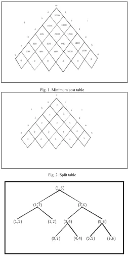
The optimal parenthesization of a matrix chain product using dynamic programming for the given sequence (5, 10, 3, 12, 5, 50, 6) is ((A1 × A2)((A3 × A4)(A5 × A6))). From the
above solution of the given problem, we can see that all possible ways of obtaining the parenthesization of a matrix chain product using dynamic programming are performed. In other words, all possible solutions are obtained, and from those solutions, the optimal solution is taken, i.e., from Step 2 to Step 5, we have selected only those solutions that provide the least or minimum value, which can be reflected in the minimum cost table, as shown in Fig. 1. The respective k values are included in the split table, as shown
in Fig. 2.
Fig. 1. Minimum cost table
Fig. 2. Split table
Backtracking is a method that helps in determining the optimal parenthesization of a matrix chain product for a given sequence by dynamic programming (i.e., it helps in obtaining the final solution, as shown below). In Fig. 3, we observe that the leaf nodes in the tree for optimal parenthesization are (1, 1), (2, 2), (3, 3), (4, 4), (5, 5), and (6, 6). However, to obtain these leaf nodes, we first check Step 5. In Step 5, the minimum value obtained is 2010, which is derived from m[1, 6], which is a combination of m[1, 2] and m[3, 6]. Hence, we consider (1, 6) as the first coordinate (Fig. 3). Now, we see that the value of m[i, j] in m[1, 6] is m[1, 2] and the value of m[k + 1, j] in m[1, 6] is m[3, 6], and thus, we check for m[1, 2] and m[3, 6] from Step 1 to 4. The desired value of m[1, 2] is found in Step 1 and that of m[3, 6] is found in Step 3. We observe that m[1, 2] has a single value (i.e., it does not have the concept of minimum values), and so, we observe that m[1, 2] is a combination of m[1, 1] and m[2, 2]. Thus, we can split (1, 2) as (1, 1) and (2, 2), as shown in Fig. 3. Now, for m[3, 6], we check in which step does it occur and we consider the minimum value. From our observation, we perceive that m[3, 6] is present in Step 3 and the minimum value is 1770. Furthermore, m[3, 6] is a combination of m[3, 4] and m[5, 6]. Thus, we can split (3, 6) as (3, 4) and (5, 6), which can be seen in Fig. 3. Finally, we check for m[3, 4] and m[5, 6]. The abovementioned procedure is followed and (3, 4) is split as (3, 3) and (4, 4), whereas (5, 6) is split as (5, 5) and (6, 6) (Fig. 3). We stop when the leaf nodes are (1, 1), (2, 2), (3, 3), (4, 4), (5, 5), and (6, 6). From Fig. 3, we can now determine the optimal solution. First, we obtain (A1 × A2).
Second, we obtain (A3 × A4) and (A5 × A6). Third, we
combine ((A3 × A4)(A5 × A6)), and finally, we combine
((A1 × A2)((A3 × A4)(A5 × A6))), which gives the final
solution.
VI. COMPLEXITY OF MATRIX CHAIN PRODUCT The time complexity of matrix chain product is O(n3), and
the space complexity of matrix chain product is O(n2) [10].
VII. CONCLUSION
Matrix chain product problem encompasses the question how the optimal classification for performing a series of operations can be determined. Moreover, matrix chain product problem is not actually to perform multiplication but simply to decide the order to perform multiplication. Thus, we have successfully determined the optimal parenthesization of a matrix chain product for a given sequence by dynamic programming using practical as well as theoretical approaches.
REFERENCES
[1] B. Bhowmik, “Simplified optimal parenthesization scheme for matrix chain multiplication problem using bottom-up practice in 2-tree structure,” Journal of Applied Computer Science & Mathematics, vol. 11, no. 5, pp. 9-14, 2011.
[2] R. Lakhotia, S. Kumar, R. Sood, H. Singh, and J. Nabi, “Matrix-chain multiplication using greedy and divide-conquer approach,” International Journal of Computer Trends and Technology, vol. 23, no. 2, pp. 65-72, May 2015.
[3] https://edurev.in/studytube/10202014-1--/5dd4be9f-8f66-40ec-b5d9-c99adae64fc4_p
[4] T. H. Cormen, C. E. Leiserson, R. L. Rivest, and C. Stein, “Introduction to algorithms,” MIT Press, July 14, 1990.
[5] www.slidefinder.net/m/matrix_mult/matrix-mult/7256761 [6] http://pt.slideshare.net/kumar_vic/matrix-mult-class17 [7] http://www.purplemath.com/modules/mtrxmult.htm
[8] http://docslide.us/documents/analysis-of-algorithms-chapter-07-dynamic-programming.html
[9] P. Gupta, V. Agarwal, and M. Varshney, “Design and analysis of algorithms,” 2nd Edition, PHI Learning Private Limited (New Delhi), ISBN-978-81-203-4663-5.