A Scenario-Driven Approach to Trace
Dependency Analysis
Alexander Egyed,
Member
,
IEEE
Abstract—Software development artifacts—such as model descriptions, diagrammatic languages, abstract (formal) specifications, and source code—are highly interrelated where changes in some of them affect others. Trace dependencies characterize such relationships abstractly. This paper presents an automated approach to generating and validating trace dependencies. It addresses the severe problem that the absence of trace information or the uncertainty of its correctness limits the usefulness of software models during software development. It also automates what is normally a time consuming and costly activity due to the quadratic explosion of potential trace dependencies between development artifacts.
Index Terms—Traceability, test scenarios, software models, Unified Modeling Language (UML).
æ
1
INTRODUCTION
I
T has been shown that the programming portion of software development requires less development cost and effort than accompanying activities such as require-ments engineering, architecting or designing, and testing [3]. It has also been shown that these accompanying activities may profoundly influence the quality of software products. As software processes have become more iterative [4], so have these activities. In an iterative process, a developer cannot discard the requirements after the design is built nor can a developer discard the design after the source code is programmed. For software development, this implies that its development artifacts are living entities that need careful maintenance. Although techniques for maintaining development artifacts are diverse, they all have in common the need to understand certain interrelation-ships between those artifacts, in particular, 1) how devel-opment artifacts may be affected by changes in other artifacts and 2) why development artifacts exist (e.g., a requirement being a rationale for a design). Traces ortrace dependencies abstractly characterize these interrelationships between development artifacts.It has been argued repeatedly that software developers need to capture traces [9], [22] between requirements, design, and code. Most methods for capturing traces, however, require extensive manual intervention [13]; even semiautomated support is rare. As a consequence, known trace dependencies are often incomplete and potentially inaccurate. This causes a dilemma since maintaining development artifacts usually requires complete and accurate knowledge of their trace dependencies. It is thus not uncommon that the lack of trace dependencies or the mistrust in their accuracy leads to their disregard in practice [6]. This reduces the usefulness of software models and
diagrams to a point where a developer may question the foundation of modeling since there is little to no value in using software models that do not consistently represent the real software system [8], [9]. Modeling trace information accurately is necessary for maintaining these various models’ consistency and the lack of it constitutes a severe problem—also known as the traceability problem [9], [12].
This work introduces a new, strongly iterative approach to trace analysis. We will show that it is possible to automatically generate new trace dependencies and vali-date existing ones. The key benefit of our approach is its automation, which must address several complicating factors:
. development artifacts are often captured informally (e.g., requirements) or semiformally (e.g., design languages such as UML [5]);
. conceptual linkages between development artifacts are often ill-defined or not understood;
. existing knowledge about traces may become invalid as their development artifacts change;
. there is a quadratic explosion in the number of potential trace dependencies.
Apparently, trace generation and validation is a com-plex, time consuming, and costly activity that may have to be done frequently due to the iterative nature of software development. Our approach avoids much of this complex-ity by requiring that the designer supply a set of test scenarios for the software system described, as well as an observable version of the software system itself. Addition-ally, a few hypothesized traces must be provided that link development artifacts with these scenarios. The essential trick is then to translate the runtime behavior of these scenarios into afootprint graph.Rules then characterize how this graph relates to the existing hypothesized traces and the artifacts to which they are linked. From these, the algorithm generates traces, usually an order of magnitude more in number than hypothesized ones. Our approach requires only a small, partially correct, initial set of trace hypotheses. Aside from generating new trace dependencies, . The author is with Teknowledge Corporation, 4640 Admiralty Way, Suite
231, Marina Del Rey, CA 90292. E-mail: [email protected]. Manuscript received Feb. 2002; revised July 2002; accepted Sept. 2002. Recommended for acceptance by M.J. Harrold.
our approach also validates existing ones. This gives developers confidence in the numerous other automated activities that rely on the existence of correct and abundant trace dependencies among evolving development artifacts. This includes, but is not limited to, consistency checking, reverse engineering, model transformation, and code generation.
2
APPROACH
2.1 Overview
As indicated above, the approach requires
1. the existence of an observable and executable soft-ware system,
2. some list of development artifacts (i.e., model elements),
3. scenarios describing test cases or usage scenarios for those development artifacts, and
4. a set of initial hypothesized traces linking artifacts and scenarios.
Scenarios are executed on the running software system to observe the lines of code they use. We refer to the lines of code used while executing a scenario as its footprint. Footprints of all test scenarios are then combined into a graph structure (called the footprint graph) to identify overlaps between them (overlaps indicating lines of code that two or more footprints have in common). A variety of rules then interpret trace dependencies in the context of these overlaps. For example, if scenario 1 uses a subset of the lines of code of scenario 2, then that overlap may indicate a trace dependency between both scenarios. If initial hypothesized traces were defined between scenario 1 and development artifact “A” and between scenario 2 and development artifact “B,” then our approach can derive that there is a dependency between “A” and “B.” This kind of reasoning can be used for:
. Trace Generation: The combined footprints in the footprint graph form a foundation for trace analyses to determine new, previously unknown trace information.
. Trace Validation: Conflicts within the footprint graph indicate inconsistencies in and/or incomple-teness of the hypothesized trace information. The extent of the generation and validation depends on the quantity and quality of the input provided. Our approach can indicate inconsistent input in the form of conflicts and incomplete input in the form of ambiguous results. An example of an ambiguous result is “A depends on B or C but not D.” An ambiguous result is still a precise statement but, semantically, it is weaker since it does not constrain the dependency between development artifacts completely (note that a nonambiguous statement defines precisely what something isandwhat something is not).
Fig. 1 gives a schematic overview of the approach. In the first step, scenarios are tested and observed. This results in observed traces that are used together with other hypothe-sized traces as input to commence trace analysis. Atomizing then combines observed and hypothesized information into the footprint graph. This graph is then subjected to various manipulations such as normalizing, generalizing, or refin-ing where modelrefin-ing information is moved around its nodes. The final graph is then interpreted to yield new trace information as well as reports about inconsistencies or incompletenesses. The trace analysis can be repeated once inconsistencies and incompletenesses are eliminated or new hypotheses become available.
In principle, the approach can detect trace dependencies among any model elements that have a relationship to code. For example, classes and methods in class diagrams, processes in dataflow diagrams, actions and activities in state chart diagrams, or use cases relate to code. It is possible to define usage scenarios for those model elements and it is possible to test those scenarios on the real system
with observable footprints. The approach cannot detect trace dependencies among model elements that do not relate to code. For example, our approach is not suitable for systems that are built out of hardware components (no code available) or for model elements that describe design decision. Our approach may be used during reverse engineering (e.g., of previously developed systems or legacy code) or it may be used during forward engineering. The latter may not be intuitive at first since a running system is required. Nonetheless, partial implementations (e.g., subcomponents), prototypes, or even simulations may be sufficient to commence analysis.
2.2 Example
To evaluate our approach, we applied it to some real-world projects such as an Inter-Library Loan system, a Video-On-Demand Client/Server application, and other case studies. One of those case studies—the Inter-Library Loan System (ILL) [1]—will be used to illustrate the approach. The ILL system automates the lending process of books, papers, and other forms of media among libraries. The system was successfully transitioned to the customer where patrons use it to order documents not available locally. ILL allows document requests to be filed via web browsers, requests that are then submitted as tagged emails to an especially dedicated email account. There, email messages are read and processed by a part of the ILL system called thePopReadcomponent.
For simplicity, this paper uses the PopRead component only which is illustrated in Fig. 2. On the left, the figure shows the functional decomposition of thePopRead compo-nent in form of a dataflow diagram (DFD) (as depicted in
the Software System Requirements Document (SSRD) [1]). In the middle, the figure shows the corresponding object-oriented design using a UML class diagram, and, finally, on the right, the figure shows a use case diagram depicting the major services thePopreadcomponent has to offer (from an user interface perspective). All three views show the PopReadcomponent in a high-level, abstract fashion. It can be seen thatPopReadreads email messages from theInbox (POP3 account), parses them, and, if the parsing is successful (OnSuccess), stores the identified requests in a back-end database (MS Access1).
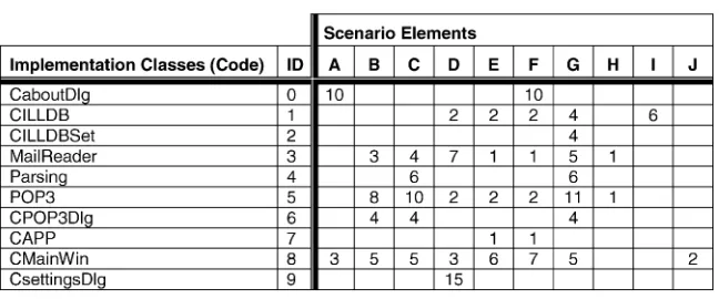
Associated with thePopReadcomponent, the ILL devel-opers also created a number of usage scenarios (Table 1). One such scenario is check for mail and unsuccessful parsing (scenario C). Another scenario is thestartup and showing the About box(scenario F).
Despite all the modeling and documentation, the ILL team failed to describe how the PopRead design elements (Fig. 2) were actually implemented (e.g., what lines of code were used by the dataflow element Add Request). Thus, trace dependencies between the code and the elements of the diagrams (dataflow, class, and use case diagrams) are missing. Table 2 lists the 10 implementation-level classes (code) of the Popread component.
Additionally, the development team did not specify how the dataflow, class, and use case diagrams related to one another (model elements in Table 3). It remains unclear what higher-level classes make up individual dataflow processes (e.g., is the class Request used in the dataflow diagram?). Even in this rather small example, some required trace dependencies are not obvious since func-tional and object-oriented decomposition is mixed.
Fig. 2. Popread Component of ILL System [1] represented in three different diagrams.
TABLE 1 Some ILL Test Scenarios
TABLE 2
Some documents, however, did capture trace informa-tion. The only problem is that we cannot safely assume their correctness. Trace information is frequently defined and maintained explicitly (e.g., in documents) which requires manual labor to keep them up to date [2]. Even if the development team took the effort to document the final trace dependencies, the activity of identifying trace infor-mation manually would still be error-prone. There exist a total of 338 trace dependencies among the given elements and it would be elaborate and time consuming to define all these dependencies manually. Our approach does use some existing trace information, despite the lack of faith in it, to generate new traces and validate old ones.
Tables 1, 2, and 3 list the scenario elements, code elements, and model elements of the ILL case study. Those tables also list short unique identification strings we have associated with each element. We will use those Ids later to more concisely refer to those elements. Table 3 additionally refers to a group ID. Groups are discussed later in Section 3.
2.3 Hypothesized, Generated, Validated, and Observed Traces
The types of trace dependencies used in our approach are depicted in Fig. 3. The figure captures the three basic ingredients required for our approach: Scenarios (Table 1), Code (Table 2), and Model Elements (Table 3). Additionally, the figure shows types of trace dependencies between them. Traces between scenarios and code (type a in Fig. 3) and traces between model elements and scenarios (type b in Fig. 3) are used as input to our approach. Both trace types a and b could be hypothesized by software developers (users of our approach); however, traces between scenarios and code can also be observed automatically during the testing of scenarios. As a result, our approach can generate new traces between model elements and scenarios (type b), model elements and code (type c), and between model elements (type d). Additionally, our approach can detect conflicts among the hypothesized traces (type b) to reason about the correctness and consistency of the input (note that we presume observed traces (type a) to be precise and correct since they are measured as will be shown in Section 3.1). Finally, our approach can pinpoint ambiguities
and incompleteness where more input is required (i.e., more hypotheses needed).
3
DETAILED
APPROACH ON
EXAMPLE
In the following, we present the details of our approach in context of the Inter-Library Loan (ILL) case study [1], a third-party software system.
3.1 Scenario Testing
The behavior of a software system can be observed using kinds of test scenarios that are typically defined during its development (e.g., acceptance test scenarios and module test cases). By executing those scenarios in the running system, the internal activities of that system can be observed and recorded. This leads to observable traces (type a) that link scenarios to implementation classes, methods, and lines of code (called the footprint). Our trace analysis approach relies on monitoring tools used for spying into software systems during their execution or simulation. Those tools are readily available. For instance, we used a commercial tool from Rational Software called Rational PureCoverage1 in order to monitor the running Inter-Library Loan (ILL) system. The tool monitored the footprint in terms of which lines of code were executed, how many times each line was executed, and when in the execution the line was covered. Testing a system or some of its components and observing the footprints is a straightforward activity. Table 4 shows the summary of observing the footprints of the 10 test scenarios from Table 1 using the Rational PureCoverage tool. The numbers in Table 4 indicate how many methods of each implementation class were used. For instance, scenario “A” used 10 methods of the class CAboutDlg and three methods of the class CMainWin. To reduce the complexity of this example, Table 4 does not display the actual methods (the information in the footprint graph shown later would be too crowded). Nevertheless, by only using classes as the finest granularity, the generated traces will still be useful. The approach remains the same if methods or lines of code are used.
Normally, observed traces are specific in nature since the repeated execution of a single test scenario may actually use different lines of code. This is caused by systems having state and depending of the current state of the system the execution of the same scenario may result in the execution of (some) different lines of code. For instance, checking for new book requests results in the execution of somewhat TABLE 3
ILL Model Elements
different lines of code if there is no email in the inbox as opposed to when there is email. To resolve this problem, we combine the traces of individual observations. For instance, if a test scenario is observed to use different lines of code after multiple executions then the observed trace is the sum of all individual observations.
Testing scenarios is normally a manual activity, but it can be automated. Scenario descriptions may be in plain English, in a diagrammatic form (e.g., sequence diagram [19]), or in a formal representation that can be interpreted by an automated testing tool. It is not important for our approach whether scenarios are tested manually or auto-matically as long as observation tools, such as Rational PureCoverage, are used to observe the footprints the testing of these scenarios make.
3.2 Finding Hypothesized Traces
Finding hypothesized traces requires reasoning in what way model elements may relate to scenarios (traces of type b in Fig. 3). Hypothesized traces can often be elicited from system documentation or corresponding models. If no documentation is available, the finding of hypothesized traces may have to be conducted manually; however, this activity becomes more automated over time since traces generated via our approach can be used as hypothesized traces in successive iterations.
An example of a hypothesized trace is the trace from scenario A to the use case About [u4] in Fig. 2. Another example is from scenario B to the dataflow elements Inbox [d1] and GetMail [d2]. Table 5 lists all hypothesized traces used in this case study. Our approach requires a small number of initial, hypothesized traces only; again hypothe-sized traces do not have to be comprehensive nor do they have to be (fully) correct. We will show later how inconsistent and insufficient trace hypotheses can be detected through contradictions and ambiguities during the trace analysis.
One of the major challenges of our approach is that most traces in Table 5 are ambiguous. For instance, the second hypothesis (check for new mail without any present) in Table 5 is a test scenario for the dataflow elements Inbox [d1] and GetMail [d2] (those are needed to read mail of the email account) and this hypothesis is ambiguous because:
1. It is uncertain whether [d1,d2] relate to code elements other than scenario B.
2. It is uncertain whether other model elements (e.g., [d5]) relate to scenario B.
3. It is uncertain what part of the observed code of B is used by model element [d1] or [d2].
Allowing ambiguity in defining hypothesized traces is very powerful for software developers because they tend to TABLE 4
Observable Scenario Footprints (Classes Used by Scenarios)
TABLE 5
have partial knowledge only. This lack of knowledge, its incompleteness and potential incorrectness, motivates the need for trace analysis. Supporting ambiguous trace hypotheses gives the users of our approach the freedom to express dependencies in a more relaxed form. This is why we also allow hypothesized traces to be expressed through inclusion or exclusion. Trace inclusion defines model elements that relate to scenarios (isScenarioFor). The trace from scenario B to model elements [d1,d2] is an example of inclusion. Exclusion defines model elements that do not relate to scenarios. Scenario B is not a scenario for class Parser [c6] (isNotScenarioFor) because no mail is found and thus no mail should be parsed. Exclusion is especially useful when it is easier to state what is not a trace dependency than what is one. Like inclusion scenarios, exclusion scenarios are ambiguous. Our approach can handle ambiguous data and still produce precise, generic results as will be shown next.
3.3 Trace Analysis
Trace analysis requires that we build afootprint graph and then manipulate it via a set of rules. The building process is called atomizing since we need to discover the largest, nonoverlapping atomic units in the graph. The rule applications comprise:normalizing,generalizing, andrefining. The aim of these rules, in essence, is to resolve the three ambiguities discussed above. This section discusses these activities in detail.
3.3.1 Atomize
Trace analysis is possible since scenarios may overlap in the lines of code they execute (their footprints). These overlaps are captured in the form of a graph structure that has as many nodes as needed to explicitly represent all possible overlaps among all scenarios (similar to concept lattices [20]). Each node in the graph depicts the largest common footprint that a set of scenarios may have in common. We refer to this graph structure as thefootprint graphand it is used as the foundation for the remaining activities in this paper. To build a footprint graph, consider the following cases:
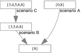
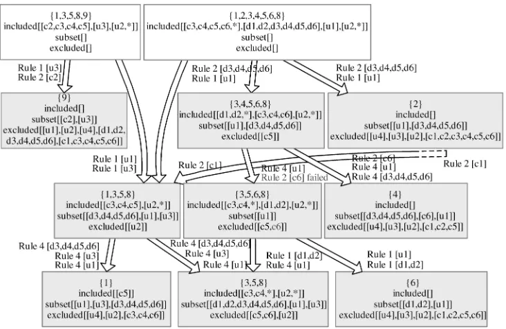
It was observed in Section 3.1, that scenario A used several methods of the implementation classes CAboutDlg and CMainWin. Scenario A thus had the observed footprint {0,8} (Table 4). Similarly, scenario B was observed to have the footprint {3,5,6,8}. To capture the footprints of both scenarios, the footprint graph is given two nodes: The first node captures scenario A with footprint {0,8} and the second node captures scenario B with footprint {3,5,6,8} (Fig. 4).
Since both scenarios overlap in the footprint {8} (im-plementation class CMainWin in Table 4), we know that both scenarios executed some common code. To capture this overlap, another node is created in the graph and that node is then declared to be achildof theparentnodes that spawned it. Fig. 4 shows the two parent nodes {0,8} and {3,5,6,8} and the figure also shows the overlap between both footprints in form of the child node {8}.
The next node added to the footprint graph is scenario C. When it is added, it is found that it overlaps with all three existing nodes. For instance, the footprint of scenario B is a subset of the footprint of scenario C. Consequently, the node for scenario B is made into a child of the node that was created for scenario C. This also made node {8} an indirect child of node {3,4,5,6,8} and no explicit edge between them needs to be added. Note that node {3,4,5,6,8} also overlaps with node {0,8}. This overlap requires no further attention since it was already taken care of through node {8}—the largest common child. It follows another property of our graph in that overlaps are captured in a hierarchical manner to minimize the number of nodes and edges in the graph. Minimal nodes and edges result in faster computation later during refinement and generalization.
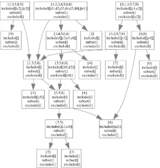
Fig. 5 depicts the complete footprint graph for the 10 scenarios in Table 1 and their observed footprints in Table 4. Adding a node to the footprint graph involves three steps.
1. The first step checks whether there is already a node with equal footprint in the graph. If one is found, then the new node is merged with the existing one (note: merging combines the attributes of the nodes which are discussed later).
2. If no equal node is found, then the second step attempts to find existing nodes that have a subset of the footprint of the new node (e.g., as {3,5,6,8} was a subset of {3,4,5,6,8}). If a subset is found, then a parent-child edge is added. Edges may also be removed if a node is inserted that is both a child and a parent of some existing nodes. For instance, later on, node {3,5,8} gets added to the footprint graph (see Fig. 5), which splits the edge between nodes {3,5,6,8} and {8}.
3. The third and final step investigates partial overlaps of footprints. If the footprint of an existing node overlaps partially with the new node, then another node with the partial overlap is created and inserted. This case occurred when node {8} was created because of a partial overlap. Since adding a node that captures a partial overlap is equivalent to adding a new node, steps 1-3 are called recursively for each partial overlap.
Finally, to represent the most atomic footprints in the graph (the individual implementation classes in this example), a node is inserted for each individual code element. The leaves of the footprint graph thus reflect the individual code elements such as {1}, {2}, or {3}.
The footprint graph in Fig. 5 also contains modeling information. Modeling information is elicited from hy-pothesized input traces (trace type b) and gets added to the graph in form ofincluded,subset, orexcludedelements (these are the attributes of nodes).
Included elements are modeling elements that are associated with a node. For instance, the trace dependency: C isScenarioFor [c3,c4,c6] in Table 5 implies the inclusion of model elements [c3,c4,c6] to the footprint of scenario C. Consequently, we add the model elements [c3,c4,c6] as included elements to the node {3,4,5,6,8}. Excluded elements are the opposite of included elements. For instance, B isNotScenarioFor [c6] in Table 5 results in the element [c6] to be excluded from footprint {3,5,6,8}.Subsetelements are used later during refinement in Section 3.3.4.
3.3.2 Normalize
Scenarios describe possible uses of model elements and are specific pieces of information. Since we would like to generate generic traces (trace types c and d in Fig. 3), we need to normalize specific information. This is accom-plished by merging all specific information about any given model elements. The assumption is that the sum of all specific behavior constitutes generic behavior. This assump-tion is in line with works from Koskimies et al. [15] or Khriss et al. [14] who also merge specific data to generate generic data. The goal of normalizing is thus to define the scope of a model element in terms of its code. The model element is then presumed to relate to a subset of the defined scope only. Normalizing resolves the first ambiguity discussed in Section 3.2.
Normalizingadds the footprints of all scenarios that are related to a given model element. It is then presumed that the remaining footprint does not relate to the given model
element. Take, for instance, the model element [c2]. It was added to the footprint graph through nodes {1,3,5,8,9} and {0,1,3,5,7,8}. This implies that footprints {0}, {1}, {3}, {5}, {7}, {8}, and {9} were used to test scenarios related to model element [c2]. Naturally, we cannot know whether [c2] belongs to all these code elements or only to a subset of them but we know that [c2] was never used with any other code element. Consequently, we define footprints {2}, {4}, and {6} as not related to [c2]. In the footprint graph, we can express this new information in form of excluded elements on nodes. We add [c2] as an excluded element to all nodes that have a subset of footprint {2,4,6}. Fig. 6 depicts a part of the footprint graph of Fig. 5 and its normalized nodes. Nodes such as {2} or {4} now have [c2] as an excluded element. Nodes such as {3,4,5,6,8} do not have [c2] as an excluded element since they also contain pieces of code (i.e., {3,5,8}) that potentially is associated with [c2].
The reasoning above is correct under the assumption that we know everything about the specific behavior of the model element [c2] (no missing scenarios). We presume this to be the case until we encounter a conflict. Indeed, our assumption about model element [c2] is incorrect since footprint element {6} also belongs to [c2]. We will show later that our approach finds a conflict related to code element {6}.
3.3.3 Generalize After Normalization
The main goal of the trace analysis is to determine how model elements relate to all nodes in the footprint graph. Ideally, we would like to know for each node what model
elements it relates to (included) and what model elements it does not relate to (excluded). The aim of generalizing is to identify the breadth of a node in terms of all model elements it could possibly support. Generalizing thus resolves the second ambiguity discussed in Section 3.2 about the uncertainty of not knowing the complete relation-ship between scenario and model elements. Generalizing is also essential for refinement later since complete knowledge about the relationship of all nodes and their model elements is required there.
The rationale for generalizing is as follows: If some knowledge exists that relates a given footprint (node) to a model element, then this knowledge is still true for any superset of that footprint because nothing gets taken away. For instance, if model elements [d1,d2] relate to node {3,5,6,8}, then we can also state that model elements [d1,d2] must relate to node {3,4,5,6,8} (its parent). Since a parent in the graph always has a larger footprint than each of its children individually, it can be defined that a parent may relate to equal or more model elements than its children but never less. In short, the parent is the union of all possible knowledge of its children.
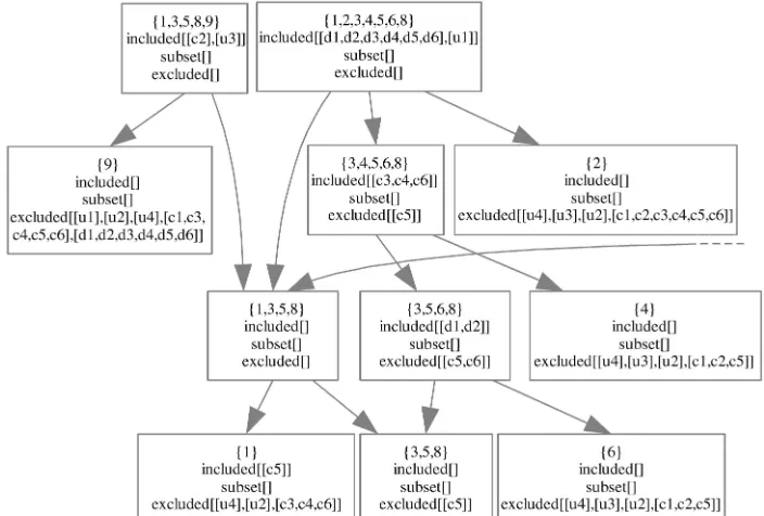
We refer to this activity as Generalizing since model information is generalized from child nodes, which are more constrained, to their parent nodes, which are more generic. Fig. 7 shows this activity on the same portion of the footprint graph as was shown in Fig. 6. We see that model elements such as [d1,d2] or [c3,c4,c6] were propagated to all their parents.
Excluded model elements are treated differently from included elements. Model elements that are excluded from a node cannot be generalized from children to parents since the exclusion constraint only holds on the given footprint and its subsets. Generalizing an excluded element is thus the reverse of generalizing an included element. Take, for instance, node {3,5,6,8} which excludes any
relationship with [c5,c6] and [u2]. We cannot be certain whether the parent still excludes those elements since the parent has a larger footprint and possibly relates to a larger set of model elements. In the reverse, however, if a model element does not relate to a given footprint, then neither may it relate to any subset of that footprint. It follows that excluded model elements can be propagated down from parents to children. For instance, model element [c6] is propagated to all its children.
At this point, the fruits of our endeavor start to pay off. By moving information around the graph, we extend our knowledge on how model elements relate to nodes. For instance, node {3,4,5,6,8} now lists the generalized model elements [d1,d2] besides the originally defined model elements [c3,c4,c6]. We have not yet completed the trace analysis, but we can already claim that model elements [d1,d2] must trace to model elements [c3,c4,c6] because they use some common code. Translated this implies that [DFD::Inbox,DFD::GetMail] has a dependency on [CD::Request,CD::Inbox,CD::Parser]. Note that know-ing a dependency between [d1,d2] and [c3,c4,c6] does not imply knowledge about their individual dependencies. For instance, does a change in [d2] cause a change in [c3], [c4], [c6] or all of them? This ambiguity is the result of the ambiguous input. We will see during refinement that ambiguities can be resolved sometimes. When ambiguities cannot be resolved, insufficient input is generally the cause. Resolving ambiguities requires manual intervention in form of defining new or refining old input hypotheses. To support the user in this task, Section 3.4 will show how our approach can pinpoint exactly where insufficient information exists and possibly what input needs to be extended or changed to resolve it. Section 3.4 will also discuss other issues related to interpreting the footprint graph.
Since all edges among nodes in a footprint graph describe subset/superset dependencies, generalizing model elements is a simple activity. Generalizing is complicated only by the computation of partial lists. Note that some nodes in Fig. 7 have lists of included elements with an asterisk at the end (“*”). The asterisk indicates that the list is presumed partial (incomplete) and model elements are assumed to be missing. Issues of partiality are important for refinement; their discussion and definition is deferred to Section 3.3.4.
Not everything went well during generalization; we also encountered a contradiction. The parent node {0,1,3,5,7,8} was declared to exclude model element [u2] (UC::Exit) but one of its children’s children {8} was declared to include [u2]. Because of generalization, these conflicting data were combined into a single node (see Fig. 8). Node {8} now has [u2] listed as an included and an excluded element–a contradiction. It is possible to trace back the origin of the contradiction and find that scenario F (startup and about) excluded [u2] (UC::Exit) and scenario J (shutdown) included [u2]. Normally, this implies that input data were incorrect and the contradiction has to be resolved by
changing scenario F, J or their initial, hypothesized traces. In this case, however, the input seems correct. Upon closer inspection, it can be seen that the trace analysis failed because it was conducted in a too coarse grained environment. Both scenarios F and J use the same implementation class {8}, but they use different methods of that class; in fact, they did not share any lines of code. Because we only consider the use of whole classes here, the input data were imprecise. If we were to repeat this trace analysis using methods as the most atomic footprints, then we would not encounter this problem. Contradictions like this are a simple form of finding inconsistent or imprecise input. Later, we will show other techniques for finding contradictions.
3.3.4 Refine
Refiningis the next activity of our approach and it induces those implications that model elements on the parent’s side might have on their children. Refinement has the goal of assigning model elements to individual code elements. Refinement addresses the third and final ambiguity discussed in Section 3.2 about the uncertainty of not knowing which parts of the code are used by what model elements. For instance, given that node {3,5,8} relates to [c3,c4] it follows that [c4] relates to a subset of {3,5,8}, but what subset?
Refiningis not as simple as generalizing and depends on whether model elements form close relationships. The notion of close relationships is used in context of all refinement rules and it essentially defines complementary, nonorthogonal modeling information. Model elements that are found within a single diagram often form a close relationship. For instance, the classes [c1,c2,c3,c4,c5,c6] describe distinct parts of the ILL system and together complement one another. The term complementary implies
Fig. 7. Generalizing some model elements for a part of the footprint graph.
that each model element can be expressed in form of individual, nonoverlapping lines of code. For instance, model element [c1] is presumed to have trace dependencies to a different part of the source code than its sibling model elements [c2,c3,c4,c5,c6]. We refer to the classes that form a close relationship as a group. In Table 3, we assigned “CD” as the unique group name for these classes. Table 3 also showed that the dataflow elements are part of another group called “DFD” and that the four use cases form groups separately. Among groups it is possible to assign same source code elements multiple times to model elements but within groups this is illegal. As such, the dataflow elements may use the same source code as the classes but two dataflow elements may not use the same portion of source code.
Note that a distinction is made between model elements that can share code and model elements that cannot share code. Our trace analysis is based on knowing that some elements may share source code but others may not. If two elements can share the same lines of code, then their refinement is not intertwined (those model elements are orthogonal to each other). All refinement rules are thus applied separately for each group. In the following, we will discuss refinement rules.
Rule 1: Refine elements to children that have no elements. The simplest refinement is between parents that have some model elements and children that have none. We refer to included elements in the parent that are not found in their children as available elements. In Fig. 7, available elements in node {1,3,5,8,9} are [c2] for group “CD,” and [u3] for group “U3;” those elements of the parent cannot be found in the children nodes {9} or {1,3,5,8}. Refinement to children that have no elements applies to group U3 only since both children have no elements of that group. Given that the model element [u3] was observed to use the footprint of the parent, it is correct to argue that each child node must cover a part of the functionality of that model
element. Consequently, we can add model element [u3] to both children (see Fig. 9). Since each child covers a part of [u3] only, it has to be added to each child node as a subset element. This reasoning is correct since we perceive model elements as atomic entities that cannot be divided.
Rule 2: Refine elements to children that have no or partial elements. Refinement scenarios may encounter lists of partial elements associated with nodes (recall Section 3.3). In Fig. 7, partial elements were indicated with a star symbol (“*”). Partial lists highlight places where model elements are presumed missing. For instance, in node {3,4,5,6,8}, the list of elements [d1,d2,*] was defined partial because one of its two children nodes ({3,5,6,8}) fully covered those model elements and the other one was empty. This raised the issue of determining to which elements the empty child node traces. One can presume that the parent has an incomplete, partial set of model elements because its children were partially investigated only. Partial is defined as follows:
. A list of model elements in a node is partial if a subset of the node’s children cover the same list of model elements and there exists at least one child that has no model element.
. A list of model elements in a node is also partial if there is at least one child node that is partial and that partial child node has the same list of model elements as its parent.
Partial lists of model elements can be treated like empty lists during refinement. An example is the list of included elements [d1,d2,d3,d4,d5,d6] in node {1,2,3,4,5,6,8}. One of its child nodes has a partial coverage of elements [d1,d2,*] and the other child nodes have no coverage. The list of available elements is the model elements of the parent minus the model elements of all its children—[d3,d4,d5,d6] for this example. Since a partial list is an incomplete list, available elements may be added to that list. The available
elements can also be added to the empty node {2} as was defined in the previous rule.
During the refinement of node {3,4,5,6,8}, we encounter another case of a contradiction. The model element [c6] is excluded in child node {3,5,6,8}, but it is refined from its parent. Since [c6] is added as a subset, it may not be an inconsistency unless no child accepts it. Recall that we attempt to create stable configurations, where the sum of the model elements of the children is equal to the model elements of the parent. If no child accepts an available model element, then there would be a contradiction. In this case, however, the other child node accepts [c6] and no contradiction is encountered. Note that this scenario also shows how input ambiguities are resolved. It was pre-viously unknown whether [c6] related to {3}, {4}, {5}, {6}, or {8}, but now it is known that it must relate to {4} because it is excluded by the others.
Rule 3: Refine elements to children that have no, partial, or complete elements. If a node contains a complete list of model elements, then no refinement rule applies to it. A complete list exists only if the list has at least one model element and it is not partial. For instance, node {3,4,5,6,8} contains the complete list {c3,c4,c6}. A parent-child config-uration where all nodes (parents and children) have complete lists of model elements is considered stable. No refinement operations can be applied on a stable config-uration. If a parent-children configuration has a mix of complete, partial, or empty lists, then this rule applies. This rule ignores complete children and adds available elements of the parent to partial and empty nodes only. The complete child is still used to compute the list of available elements. Fig. 10 shows the application of Rule 3 in context of the nodes {0,1,3,5,7,8}, {1,3,5,7,8}, and {0,8} (see also Fig. 5). One child node {1,3,5,7,8} has a complete list [c1,c3,c4,c5] and the other child node {0,8} is empty (recall that refinement is done for each group of closely-related elements separately). The only available element [c2] is thus refined to node {0,8} but not to node {1,3,5,7,8}.
It must be noted that there may exist cases where it would be semantically correct to propagate model elements to complete children since our notion of completeness is only valid if complete and correct input data were provided. Given that input data are likely ambiguous, incomplete, and possibly incorrect, it follows that our notion of completeness may not hold always. We take a conservative stance here by not propagating model ele-ments in case of uncertainty. It is always correct to
propagate [c2] to node {0,8} but possibly incorrect to propagate it to {1,3,5,7,8}. Conservative rules avoid false positives but at the expense that not all potential trace dependencies are determined. Nonetheless, our graph has the benefit of redundancy that may compensate for conservative refinement rules in some cases. Consider the example of node {3,5,6,8} which contains the presumed complete list {d1,d2}. Its child {3,5,8} has two parents and through the other parent {1,3,5,8}, it receives the elements {d3,d4,d5,d6}. Those elements can be generalized later and, thus, will reach the presumed complete parent, extending it with new information.
It is valid to argue similarly for why only available elements should be added to children and not all elements of a parent. There are situations where it would be semantically correct to propagate all elements a parent has to offer irrespective of model elements already used by some children. Again, we prefer to be conservative and only propagate those elements of the parent that have not been assigned to children. Fig. 10 shows one example of the danger of propagating too much. The model element [u4] is considered complete in node {0,8}. Through generalization, it was added to its parent node and there it was determined to be partial (star symbol). Would we ignore this informa-tion and attempt to refine [u4] to node {1,3,5,7,8}, then we would introduce an error since the model element [u4] does not trace to footprints such as {1}, {3}, or {5}.
Rule 4: Refine subset elements. Subset elements can also be refined from parent nodes to child nodes. Their refinement is analogous to Rules 1-3 and also results in subset elements. The only difference lies in the computation of available elements. Here, available elements are the subset elements of the parent minus the included elements of the children. Subset elements of the children are not subtracted because only a subset of them actually belong there. Note that our refinement rules are defined in a manner that avoids race conditions. It neither matters in what order refinement rules are applied nor in what order nodes are visited.
3.3.5 Generalize Specific after Refinement
This generalization activity is identical to the one discussed in Section 3.3.3. It generalizes elements from children that had two parents and potentially received complementary information (i.e., node {3,5,8}).
3.4 Result Interpretation
In a final activity, the footprint graph is interpreted by traversing its nodes to elicit new trace information or to find contradictions. This activity investigates each node of the graph to determine the model elements that are associated with it. Depending on the state of the association of a model element with a node (included, subset, or excluded), it is then possible to infer trace dependencies. As mentioned earlier, our approach can generate new trace dependencies of types b, c, and d (recall Fig. 3) and, if contradictions are encountered, our approach can invalidate hypothesized trace dependencies of type b.
3.4.1 Trace Generation
The rationale for trace generation is simple: If multiple model elements share some lines of code (footprint), then there has to be a trace dependency among them. Since model elements associated with nodes are places where those model elements share code, we can derive trace dependencies by investigating them. For instance, through node {3,4,5,6,8}, we learn that model elements [c3,c4,c6] must trace to model elements [d1,d2] plus a subset of ½ðd3jjd4jjd5jjd6Þ (subset notation implies zero or more elements of [d3,d4,d5,d6]). If the code for {3,4,5,6,8} is changed, then it may affect both½d1;d2;ðd3jjd4jjd5jjd6Þand [c3,c4,c5]. In reverse, if [c3,c4,c5] is changed, then this affects the code {3,4,5,6,8}. Given that we know that a change to {3,4,5,6,8} requires a change to ½d1;d2;ðd3jjd4jjd5jjd6Þ, we can infer that a change to [c3,c4,c5] also requires a change to ½d1;d2;ðd3jjd4jjd5jjd6Þ—a trace dependency. This kind of reasoning can be repeated for all nodes but one can do more. Table 6 describes rules on how model elements can be interpreted in the context of leaf nodes (nodes without children). Leaf nodes are the most atomic nodes in the graph and it is presumed that each leaf node may trace to only single model elements of same groups (recall that we disallow model elements of the same group to share code). Table 6 lists the number of included, subset, and unknown elements on the left. Included and subset elements can be derived directly out of the leaf nodes. For instance, node {4} has no included element and one subset element [c6]. Unknown elements are total elements of a group minus included, subset, and excluded elements. For instance, the model elements in group “CD” are [c1,c2,c3,c4,c5,c6]. We know that [c6] is subset and [c1,c2,c5] are excluded. The relationships of elements [c3,c4] to node {4} are thus unknown. In case of node {4}, Table 6 allows the subset element [c6] in node {4} to be upgraded to an included element since it is the only element that has claimed interest in that node.
Table 6 also shows that some combinations of included, subset, and unknown elements are considered indications for incompleteness or inconsistency. For instance, if a leaf node has no included element but two or more subset elements (e.g., [c3,c4] in node {5}), then the provided input hypotheses were insufficient to make a more precise statement. Recall that insufficient (incomplete) input data generally yield ambiguous results. Examples for inconsis-tencies are leaf nodes that have more than one included element or one included element and one or more subset elements. These examples indicate cases where multiple
model elements of the same group claim a portion of source code as their own.
If the rules in Table 6 are applied to all leave nodes in the footprint graph, then Table 7 is the result. The table contains an “I” if an element is included, an “S” if an element is subset, an “X” if an element is excluded, “?” if the relationship of that element is unknown, and “(I)” if a model element is both included and excluded. Some model elements were upgraded from subset to included (i.e., [c2]) and some model elements remain ambiguous (i.e, [c3]). In case of code element {6}, we encounter a contradiction: No single subset or included model element was identified but unknown ones exist. This implies that node {6} was observed to belong to some classes but it was never determined what classes those may be. This case is a contradiction because the given input was overconstrained and, thus, likely incorrect. It may be necessary to investigate all hypothesized input traces related to the parent’s footprint to understand the cause of the conflict.
The trace analysis was very effective in assigning classes and use cases to code elements. Dataflow elements are still very ambiguous. Based on Table 7, one can derive new trace dependencies such as the following:
. Use case UC::Exit [u4] traces to the class CD::User-Interface [c2].
. Class CD::Parser [c6] traces to a subset of the dataflow elements DFD::ParseRequest [d3], TABLE 6
Interpreting Model Elements in Leaf Nodes
TABLE 7
Individual Model Elements and Their Traces to Implementation Classes (Code) (“I” ... Included; “S” ... Subset; “X” ... eXcluded;
DFD::AddRequest [d4], DFD::DeleteMail [d5], or DFD::DatabaseBackEnd [d6].
. Use case UC::Settings [u3] traces to the classes CD::UserInterface [c2], CD::Request [c3], CD::Inbox [c4], CD::DBBackEnd [c5] (may seem nonintuitive but [c3,c4,c5] are reconfigured upon completion of Settings).
. Class CD::UserInterface [c2] traces to the implemen-tation classes {0}, {8}, {9}, and possibly to {7}.
. Class CD::PopreadApp [c1] does not trace to any dataflow elements.
. Dataflow element DFD::DeleteMail [d5] does not trace to implementation classes {0,7,9}.
The above list of generated traces shows previously unknown trace dependencies among model elements (trace type d in Fig. 3) and between model elements and code (trace type c). The generated traces cover both inclusion and exclusion. Table 7 also contains some counterintuitive trace observation such as UC::About [u4] has some trace dependencies with at least one dataflow element ½ðd1jjd2jjd3jjd4jjd5jjd6Þ. This observa-tion is counter-intuitive because displaying the about dialog box should have nothing in common with the dataflow diagram for checking email requests. This observation arose because [u4] and the dataflow elements share the implementation class {8}. As we discussed in Section 3.3.3, both model elements actually use different methods of that class and thus no factual trace depen-dency exists. If we were to repeat the trace analysis using methods or even lines of code as the most atomic code elements, then we would not encounter this problem.
Although it is possible to generate substantial new trace information through the leaf nodes in Table 7, they do not replace the other nodes in the footprint graph. For instance, in Table 7, we would find a trace dependency between [c2,c3,c4,c6] and a subset of½ðd1jjd2jj3jjd4jjd5jjd6Þ. Earlier in this section, we showed that through node {3,4,5,6,8} we can derive a more precise statement in that [c2,c3,c4,c6] traces to both [d1] and [d2] plus a subset of ½ðd3jjd4jjd5jjd6Þ. The latter statement is less ambiguous. Deriving trace depen-dencies out of nodes has to be done carefully:
. It is potentially incorrect to derive trace dependen-cies among subset lists. Subset elements contain elements that are only partially correct. Deriving a trace dependency between two partially correct lists has the downside that the incorrect portions are related as well. For instance, it is incorrect to
define a trace between [(c2)] and½ðd3jjd4jjd5jjd6Þin node {3,4,5,6,8}.
. It is potentially incorrect to derive trace dependen-cies among partial lists: Partial lists are also incomplete. Given that two partial lists may be incomplete in distinct ways, it might be incorrect to relate them. For instance, there is no trace depen-dency between [u2,*] and [d1,d2,*] in node {3,4,5,6,8}. Keeping the above constraints in mind, one can generate dependencies from the nodes in the footprint graph using the algorithm in Fig. 11. The algorithm takes an arbitrary list of source elements as an input (i.e., source = [c2]) and produces new trace dependencies between those source elements and elements of other groups. Since a dependency has a source and a destination, the algorithm aims at finding all possible destinations to the given source. To do so, it locates all nodes in the graph that contain the given source element(s) (i.e., nodes {0}, {8}, {9}, {0,8} for [c2]). The variable excluded is computed by finding the intersection of excluded elements of all nodes ([u2] is the only excluded element common to {0}, {8}, {9}, {0,8}). No trace dependency exists between source and excluded ([c2] does-not-trace-to [u2]). The variable destina-tion is the union of all included/subset elements in nodes ([u1], [u2], [u3], [u3], ½ðd1jjd2jjd3jjd4jjd5jjd6, [u1,*], [u2,*], [u3,*]); excluding those elements that are defined partial but contain all elements of group (e.g., [u1,*], [u2,*], and [u3,*] are defined partial but they already contain all elements of their group). Since the destination may contain elements of separate groups, we define trace dependencies between source elements and the groups of destination elements separately ([c2] traces-to [u1]; [c2] traces-to ½ðd1jjd2jjd3jjd4jjd5jjd6Þ; etc.). The variablecodeis the union of code elements of all given nodes ({0,8,9} for [c2]). A trace dependency is thus between source and code ([c2] traces-to [0,8,9]). Finally, the variablescenariosis the union of all scenarios in given nodes (scenario A for {0,8}; scenario J for {8}). A final trace dependency is thus between source and scenarios ([c2] traces-to [J,A]). The following is the complete list of generated trace depen-dences for model element [c2]:
LIST OF DEPENDENCIES AMONG MODEL ELEMENTS: Dependency:
[c2] traces-to [(d1||d2||d3||d4||d5||d6)] Dependency: [c2] traces-to [u1]
Dependency: [c2] traces-to [u2]
Dependency: [c2] does-not-trace-to [u2] Dependency: [c2] traces-to [u3]
Dependency: [c2] traces-to [u4]
LIST OF DEPENDENCIES BETWEEN MODEL ELEMENTS AND CODE:
Dependency: [c2] traces-to [0,8,9]
LIST OF DEPENDENCIES BETWEEN MODEL ELEMENTS AND SCENARIOS:
Dependency: [c2] traces-to [J,A]
3.4.2 Trace Validation
Based on the state of the footprint graph, it is possible to infer incompleteness and inconsistencies. Previous sections pointed out most rules for detecting them. The following briefly summarizes those rules.
Incompleteness. Incompleteness in context of our approach implies that insufficient input data were given and the exact nature of trace dependencies could not be inferred in all cases. Incomplete input data leads to ambiguous results. Incompleteness can be measured in how well the leaf nodes in the graph relate to individual model elements. Consider, for instance, the leaf node {5}. Although our approach was successful in matching code elements to classes, it was not able to determine whether code element {5} traces to model element [c3] or [c4]. A simple tiebreaker would be to define a new input hypoth-esis relating [c3] to {5}. Through leaf nodes, incompleteness can be detected easily and potential solutions are obvious (i.e., select from list of included/subset elements).
Inconsistencies. Inconsistencies in context of our approach imply that conflicting constraints where given as input and no solution is possible that would satisfy all given constraints. We can detect the following types in inconsistencies:
1. If a model element is included and excluded in the same node (i.e., [u2] in {8}): This inconsistency can be traced back to its origin by investigating how the contradicting model elements converged onto that node.
2. If a model element does not trace to any code: Since we presume that every model element must have some individual piece of code, no trace dependency from a model element to code is a conflict (our example has no such conflict).
3. If a leaf node contains more than one included element of the same group: This is an inconsistency because model elements of the same group cannot share code.
4. If the model elements of the parent are not equal the sum of all model elements of its children (included + subset): This inconsistency can occur only if all children are presumed complete (nonpartial) but the parent has available elements not found with any child (not encountered in our example).
5. If a leaf node (= code element) does not relate to any model element of a given group but has unknown elements of that group: Recall that unknown elements are elements that are neither included nor excluded. They imply the existence of a parent that used the footprint in context of some model elements
of that group. Since it was never determined how the elements of the parent refer to the conflicting child, we may conclude that the input hypotheses were overconstrained.
4
VALIDATION
Besides validating our approach on smaller or hypothetical examples, our approach was also validated on several large-scale, real-world case studies such as the Library Loan System (ILL) or a Video-On-Demand system (VOD). Furthermore, in our studies, we subjected our approach to different input hypotheses and scenario observations to evaluate its responses. This section discusses observations made about quality, incorrect results, and other issues.
4.1 Quality of Results
Our example started out with only a few hypotheses and during the course of analyzing the given information our approach was able to generate new trace information and invalidate existing ones (i.e., initial, hypothesized traces). Upon inspecting the quality of the newly generated traces, we indeed find that they fit the problem well. A major concern was whether our approach produced incorrect results (false positives). We observed that the false positives produced were all caused by incorrect input data. We also found that in most cases our approach was able to indicate incorrect input through conflicts detected. In context of the ILL system, our approach detected two conflicts. The first conflict was about model element [u2] and its concurrent inclusion and exclusion. The second conflict was about leaf node {6} and the problem that it was not determined what classes it traces to. The first conflict could be pinpointed and resolved easily. The second conflict required the inspection of the parent and siblings of node {6} to determine the cause of the problem. It is future work to improve the automatic localization and reasoning of the origin of conflicts.
The main reason why we avoid false positives is because of our conservative set of rules. However, conservative rules have the effect that some potentially correct trace dependencies are discarded. For instance, model element [c2] was determined to trace to code elements {0}, {8}, and {9} and to not trace to {2}, {4}, {6}. If the input hypotheses were correct, then one could be certain of these results. Nonetheless, our approach was uncertain about code elements {1}, {3}, {5}, and {7}. Given that our rules were conservative our approach neither included nor excluded them. It is thus possible that [c2] traces to more code elements than {0}, {8}, and {9}.
4.2 Quantity of Results
precise and six ambiguous input hypotheses and the case study used 12 scenario observations. Our approach gener-ated over 200 precise and ambiguous results—a ratio of about 10 new traces per input trace. We observed similar gains in other case studies.
4.3 Complexity of Trace Analysis
The trace analysis activity is not very expensive computa-tionally. The activities of normalizing, generalizing, and refining are linear complex with O(n), where n is the number of nodes in the footprint graph; the activity of interpreting is O(n2). In the worst case, the number of nodes
in the graph could be as high as number of code elements+ (number of scenarios)2 where every scenario overlaps with
every other scenario in different ways—a rather unlikely case. The case study in this paper only had 20 nodes for 10 scenarios and 10 code elements; all other case studies were within this range (e.g., the video-on-demand system had 65 nodes for 185 code elements and 28 scenarios).
The complexity of trace analysis is similar if more granular code elements are used. Recall an earlier conflict where model elements were linked because they used the same implementation classes but different methods within those classes. Such cases can be avoided if the trace analysis is repeated using methods as the most granular code elements. The trace analysis does not change and it does not become much more expensive computationally. For instance, in context of the video-on-demand system, 20 implementation classes produced 40 nodes, whereas 170 methods produced 75 nodes. Still there are other computational aspects to consider. For instance, handling 170 methods during trace analysis costs more memory and computation than handling 20 implementation classes (i.e., comparison of 170 methods would be more expensive than the comparison of 20 implementation-level classes).
4.4 Required Quantity of Input Data
We found that our approach only requires a small amount of input data in order to function. Trace analysis can be performed at any time using any set of input data. If less input data are given, our approach will produce ambiguous results. Initially, our approach does not indicate how much or what input data are required to produce precise results. After the completion of the first iteration of the trace analysis, this changes and the existence of ambiguities in leaf nodes indicates very precisely what more information is required to make the results better.
4.5 Required Degree of Correctness of Input Data We observed that the trace analysis is less constrained when less input is given. Incorrect input is more likely to remain undetected in a weakly constrained environment. Since undetected, incorrect input is trusted as correct, such input may produce (partially) incorrect results. The advantage of our approach is in its iterative nature. Our approach points out where more information is needed (ambiguity) and the more hypotheses are added the more constrained the environment becomes. This constrains the analysis and makes it increasing likely to detect incorrect input.
5
DISCUSSION
5.1 Semantic Meaning of a Trace
Our approach generates and validates trace dependencies but our approach does not define the semantic meaning of those trace dependencies. For instance, our approach is capable of finding traces between some dataflow elements and some code indicating what code may have to be changed with a change in those dataflow elements or indicating what dataflow elements may become invalid if the code changes. Given that this trace spans between dataflow elements and code, it gives rationale why the code is there. It follows that semantic meaning of trace dependencies can be inferred through the semantic differ-ences among the development artifacts they bridge. The implication is that we see traces as neutral entities—they simply describe dependencies; however, how to interpret dependencies or how to use them depends on the development artifacts they bridge.
5.2 What if no Code is Available?
It is also possible to use our approach if no observable software system exists. For instance, we experimented with simulators that could replace running software systems. Scenarios can then be tested and observed in context of the simulated system. In case no simulation exists, it is also possible to hypothesize about the footprint of scenarios. For instance, one could use a model of the software system and hypothesize the impact of testing a scenario onto the model. The trace analysis would be identical, but the downside is that conflicts may also arise out of wrongly hypothesized observations.
5.3 Traces among Model Elements that form Close Relationships
Our approach does not generate traces among model elements that form close relationships. For instance, our approach will not indicate a trace dependency between two classes of the same class diagram. This is primarily because it is presumed that they trace to different pieces of the source code. We do not believe that this weakens our approach because elements that form close relationships are usually contained in a single diagram and that diagram should already describe the dependencies among its elements.
5.4 Legacy Systems and COTS Components
The ILL is a third-party software system and we were not involved in its development. Furthermore, we did not have the benefit of interacting with its developers while performing this study. Our situation is therefore compar-able to the situation of any development team that is asked to reuse old legacy systems. While analyzing the ILL system, we had to use a number of trial-and-error steps to find hypothesized traces that result in only few contradictions. Our approach supports this type of explorative form of trace detection since success can be measured in the number of ambiguities and conflicts produced.
POP3 server. Furthermore, Microsoft Access1 was used to store book requests in a back-end database. Although we were not able to observe the internal workings of those components, our approach nevertheless was able to generate trace information to them since observable wrappers covered those COTS packages. Those wrappers thus became substitutes for the COTS packages.
5.5 Functional and Object-Oriented Decomposition An interesting feature of the chosen example is that it was implemented in C++ but mixed functional and object-oriented decomposition. As such, the parsing component was implemented in a functional manner, whereas the rest of the system was implemented in an object-oriented manner. To complicate matters, the model also mixed functional and object-oriented styles (dataflow diagram versus class diagram). The circumstance that our approach used the source code as a foundation for analysis ignored these conceptual boundaries.
6
RELATED
WORK
Current literature contains ample publications about the need for traceability [9], [22]; however, few publications report work in generating or validating trace information.
The works of Gotel and Finkelstein [9] discuss the traceability problem and why it still exists. One reason they believe to be the main cause is the lack of prerequirements traceability. They argue that tracing requirements only, as many do, is not sufficient since requirements do not capture rationale. We agree with their point, but we also believe that the lack of traceability throughout the entire software development life-cycle is another significant reason. Our work enables the traceability among all software develop-ment artifacts and, thus, is a potential solution to the traceability problem. We also demonstrated in context of the video-on-demand case study that our approach can generate prerequirements trace dependencies [7].
Lange and Nakamura present a program for tracing and visualization [16]. They take a similar approach to ours since they observe runtime behaviors of object-oriented software systems. They do this to capture, visualize, and analyze trace information. The main difference is that their emphasis is on how to best visualize trace information. Consequently, they do not perform trace analysis to generate or validate trace information.
Pinheiro and Goguen [18] took a very formal approach to requirements traceability. Their approach, called TOOR, addresses traceability by reasoning about technical and social factors. To that end, they devise an elaborate network of trace dependencies and transitive rules among them. Their approach is mostly useful in the context of require-ments tracing and, thus, ignores the problem of traceability among development artifacts in general. Their work also ignores the problem of how to generate and validate trace dependencies among development artifacts that are not defined formally and completely.
Murphy et al. [17] present a different but formal technique where source code information is abstracted to match higher-level model elements. They use their abstrac-tions for consistency checking between model and code. In
particular, they aim at finding how abstraction and model diverge. Although their aim is to closely relate model and code, they presume the existence of mapping rules between them. Their work is thus only useful if complete trace dependency knowledge exists.
Concept analysis is a technique similar to ouratomizing activity. Concept analysis (i.e., as used for the reengineering of class hierarchies [20]) provides a structured way of grouping binary dependencies. These groupings can then be formed into a concept lattice that is similar in nature to our footprint graph. It is unclear, however, whether concept analysis can be used to group and interpret three-dimen-sional artifacts (code, scenarios, and model elements) as required in the footprint graph.
The approaches of Haumer et al. [11] and Jackson [13] constitute a small sample of manual traceability techniques. Some of them infer traces based on keywords, whereas others use a rich set of media (e.g., video, audio, etc.) to capture and maintain trace rationale. Their works only provide manual processes, but do no automate trace generation and validation (except for capturing traces). As our example has shown, trace generation for even a small system can become very complex. Manual trace detection, though effective, can thus become very costly. Despite some deficiencies of the approaches above, their techniques are useful since they cover trace generation issues outside our domain or could be used to derive hypothesized trace information needed for our approach.
Our work also relates to program slicing. Our approach observes the source code of a software system according to test scenarios executed on it. This activity is similar to slicing, where the source code is observed (sliced) according to some property or rule. The main purposes of slicing are to understand code dependencies, support debugging, and to manipulate code to introduce or eliminate some prop-erty. Slicing thus divides source code and then recomposes it in a different manner to add or remove some desired or undesired properties. Our approach does not have the goal of manipulating the source code or the model. Our approach simply uses observations made on both for transitive reasoning.
Our work also relates to the research on separation of concerns [21]. The aim of separation of concerns is to elicit modeling information or code that relates to individual concerns. For instance, a concern could be a nonfunctional requirement that has to be satisfied. By separating concerns, it is hoped that it becomes possible to manipulate them without affecting one another. Our approach is a natural complement to separation of concerns. We believe that it is possible to define scenarios based on concerns. By using our approach, one can then find model elements and source code related to individual concerns.

![Fig. 2. Popread Component of ILL System [1] represented in three different diagrams.](https://thumb-us.123doks.com/thumbv2/123dok_us/7874362.1306272/3.612.119.448.69.194/fig-popread-component-ill-represented-different-diagrams.webp)