The Role of NWP Filter for the Satellite Based
Detection of Cumulonimbus Clouds
Richard Müller1* ID, Stephane Haussler1and Matthias Jerg1,
1 German Weather Service, Frankfurter Str 135, 63067 Offenbach, Germany
* Correspondence: Richard.Mueller@dwd.de; Tel.: +49-(0)69-8062-4922
Abstract:The study investigates the role of NWP filtering for the remote sensing of Cumulonimbus 1
Clouds (Cbs) by implementation of 14 different experiments, covering Central Europe. These 2
experiments compiles different stability filter settings as well as the use of different channels for 3
the InfraRed (IR) brightness temperatures. As stability filter parameters from Numerical Weather 4
Prediction (NWP) are used. The brightness temperature information results from the IR SEVIRI 5
instrument on-board of Meteosat Second Generation satellite and enables the detection of very cold 6
and high clouds close to the tropopause. The satellite only approaches (no NWP filtering) result 7
in the detection of Cbs with a relative high probability of detection, but unfortunately combined 8
with a large False Alarm Rate (FAR), leading to a Critical Success Index (CSI) below 60 %. The false 9
alarms results from other types of very cold and high clouds. It is shown that the false alarms can be 10
significantly decreased by application of an appropriate NWP stability filter, leading to the increase 11
of CSI to about 70 % . A brief review and reflection of the literature clarifies that the this function 12
of the NWP filter can not be replaced by MSG IR spectroscopy. Thus, NWP filtering is strongly 13
recommended to increase the quality of satellite based Cb detection. Further, it has been shown that 14
the well established convective available potential energy (CAPE) and the convection index (KO) 15
works well as stability filter. 16
Keywords:cumulonimbus; thunderstorms; stability filter; aviation 17
1. Introduction 18
Cumulonimbus clouds (Cb) originate from rapid vertical updraft of humid and warm air enforced 19
by constraint forces caused e.g. by mountains, heating or cold fronts. The fast cooling of the air with 20
rising height leads to optically thick and very cold clouds, referred to as cumulonimbus clouds (Cbs), 21
which are usually accompanied by lightning, heavy precipitation, hail, and turbulence. Early and 22
reliable prediction of Cb clouds is therefore of great importance for weather forecasts and warnings, in 23
particular for aviation, as Cb clouds (thunderstorms) constitute one of the most important natural risks 24
for aircraft accidents. An accurate Cb detection and short term forecast enables cost-efficient planning 25
and use of alternative routes, increasing flight safety. 26
Yet, the reliable simulation of convective cells and Cbs by means of numerical weather prediction 27
is still a very difficult task. Thus, observational data plays a pivotal role for the accurate detection and 28
short term forecast of Cbs. Over ocean and a vast number of countries, which are not well equipped 29
with precipitation RADARs, satellites are in addition to global lightning ground based networks the 30
only observational source for the detection of Cbs, e.g. [1]. As a result of the thermodynamics involved 31
in the generation of Cbs they are optical thick and their tops are located close to the tropopause. 32
Therefore, from a satellite perspective they are characterized by very cold brightness temperatures 33
corresponding to high cloud top heights (CTH). 34
Thus, cloud top height is on option used as a straightforward method to provide information 35
about the risk for cumulonimbus cloud occurrence as operated by e.g. NCAR ([2] and references 36
therein). The cloud top height can be derived from the brightness temperature (BT) in the atmospheric 37
window channel (InfraRed 10.6), which corresponds in good approximation to the temperature of the 38
cloud top for Cbs. A NWP based profile of the atmosphere can then be used to link the temperature 39
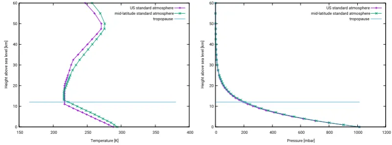
to the height of the cloud top, see figure1for an example of an atmospheric profile. A more detailed 40
discussion of methods for the estimation of CTH are presented in [3].
0 10 20 30 40 50 60
150 200 250 300 350 400
H ei gh t a bo ve s ea le ve l [ km ] Temperature [K]
US standard atmosphere mid-latitude standard atmosphere tropopause 0 10 20 30 40 50 60
0 200 400 600 800 1000 1200
H ei gh t a bo ve s ea le ve l [ km ] Pressure [mbar]
US standard atmosphere mid-latitude standard atmosphere tropopause
Figure 1.Left hand: The image shows the relation of the height above sea level and the temperature
in the atmosphere for the US standard atmosphere and a standard atmosphere for mid-latitude summer. Diagrammed is also the height of the tropopause, which "separates" the troposphere from the stratosphere. Right hand: Relation between pressure and height for the same profile.
41
Another simple, but widely used method is that applied in the Global Convective Diagnostics 42
approach [4] and [2]. The method uses the brightness temperature difference between the 6.7µmthe 43
11.6µminfrared satellite channel, the former is also referred to as water vapour channel, cause of 44
the large water vapour absorption bands. If the difference exceeds 1 degree it is assumed that the 45
observed cloud is a cumulonimbus cloud. The physical background of this approach has been already 46
discussed in 1997 by Schmetz et al. [5]. They investigated the potential of satellite observation for the 47
monitoring of deep convection and overshooting tops. They found that the brightness temperature 48
of the water vapor channel (5.7-7.1µm) can be larger (warmer) than that of the IR window channel 49
(10.5-12.5µm). They demonstrated by radiative transfer modeling (RTM) that the larger brightness 50
temperatures (BT) in the WV channel are due to stratospheric (tropopause) water vapor, which absorbs 51
radiation from the cold cloud and subsequently emits radiation at higher temperature (warmer), as 52
the temperature increases in the stratosphere, see figure1. The effect is largest when the cloud top 53
is at the tropopause temperature inversion. Optical thick high clouds cover the tropospheric water 54
vapor and only the emission from the stratospheric water vapor contributes to the radiance observed 55
by the satellite instrument. In contrast, for lower clouds the tropospheric water vapor above the clouds 56
absorbs the radiation and the emitted radiation is colder than the absorbed. It is therefore obvious that 57
the temperature difference increases with increasing cloud height. 58
The effect discussed by [5] occurs also if the difference of the two water vapor channels are used. 59
The use of this combination is possible since the launch of Meteosat Second Generation satellites, which 60
has the Spinning Enhanced Visible and InfraRed Image (SEVIRI) instrument on-board. This instrument 61
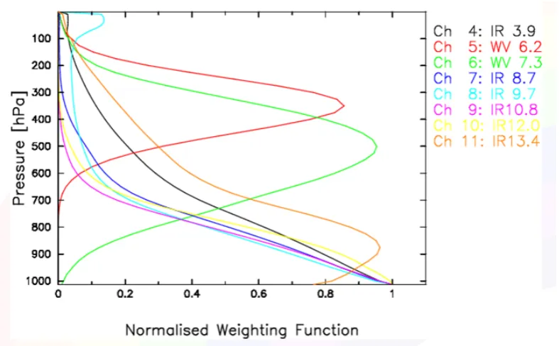
is equipped with additional channels in the Infrared (IR). The normalized weighting function of the 62
SEVIRI IR channels is diagrammed in Figure2for clear sky. 63
Note, that the water vapor channel at 6.2 µm receives significant contributions from the 64
stratosphere, which are larger than the equivalent contributions of the WV channel at 7.3µm. Thus, 65
the mechanism discussed by Schmetz et al [5] works also well for the difference of the water vapor 66
channels. 67
A slightly different approach is used by the Nowcasting Satellite Application Facility NWC-SAF. 68
This method is based upon an adaptive brightness temperature thresholds of infrared images [6]. 69
Further, cloud classification methods have been developed which use texture information of the visible 70
Figure 2.The image shows the normalized weighting function of MSG for clear sky , source Eumetrain
NRL Cloud Classification (CC) algorithm [7] is one example. It is used by the Oceanic Weather Product 72
Development Team to assist in the accurate detection of deep convective clouds. Another example 73
is the Berendes cloud mask [8]. However, in both methods visible channels are utilized and they are 74
therefore not applicable during night. Thus, these approaches are not sufficient to provide a day and 75
night service needed by aviation. Finally, there exists a commercially offered software package, which 76
has been developed and validated by Zinner et. al [9] and references therein. 77
All these approaches use information from the IR region for the satellite based detection of Cbs. 78
However, not only Cbs are optically thick and cold, but also other clouds, which can lead to serious 79
false alarms. As briefly discussed in [2] these false alarms might be reduced by the implementation of 80
an stability filer from NWP. 81
To the knowledge of the authors the above mentioned methods do either not apply an NWP filter 82
(e.g. [6–9] or did not provide an extensive analysis and discussion of NWP filtering ([2,4]), e.g. by 83
implementation of different experiments. Further, the role of NWP filtereing is not reflected in relation 84
to IR spectroscopy. Thus, the central novel aspect of this work is the extensive discussion and analysis 85
of NWP filtering for the quality of satellite based Cb detection, including a reflection of SEVIRI IR 86
spectroscopy as alternative. 87
2. The method 88
The difference of the brightness temperature of the WV channels of the SEVIRI instrument on 89
board of the Meteosat Second Generation satellite (MSG) is used as starting point of the study and 90
in the majority of the experiments. This approach is based on the method discussed in [5] and more 91
relevant to present times applied by e.g. [4] and [2]. However, in our method, the WV 7.3 channel is 92
used instead of the atmospheric window channel for the calculation of the brightness temperature 93
difference. 94
Further, in contrast to [2] a threshold of -1Kis applied in the first experiments. However, further 95
experiments are performed with different thresholds. As the temperature signal of Cbs is not only 96
apparent in the WV channels the performance of further channels combinations are investigated in the 97
For the stability filter the well established convective available potential energy (CAPE) is used 99
[10]. CAPE is the amount of energy a parcel of air would have if lifted a certain distance vertically 100
through the atmosphere. It is effectively the positive buoyancy of an air parcel. 101
As a supplementing filter to CAPE the Totals Total (TT) index has been used. It is defined as:
TT=T850+Td850−2∗T500 (1)
hereTis the temperature,Tdis the dew point temperature and the numbers provide the respective 102
pressure level. 103
Further, the KO index defined in equation2have been applied in further experiments;
KO= 1
2 ·(θe700 +θe500 −θe1000 −θe850) [K] (2) hereθeis the pseudo potential temperature in Kelvin for the different pressure levels 1000, 850, 700
104
and 500 hPa. 105
The "stability" filters (CAPE and TT) for the first experiments (up to experiment 9) are taken from 106
the comprehensive Earth-system model developed at ECMWF in co-operation with Météo-France. 107
A detailed documentation of can be found at the ECMWF web-page, see [11] and concerning the 108
convection part in [12]. The thresholds for the NWP stability filters (CAPE and TT) have been varied 109
in the experiments (experiment 7,8), but for the reference experiment 1 they have been set to CAPE=60 110
and TOTALX=50. Within case studies (visual inspection) other "filter" variables provided by ECMWF 111
have been investigated but have been excluded in the experiments due to their comparatively poor 112
performance. 113
In order to investigate the sensitivity of the NWP filtering on the chosen NWP model CAPE has 114
been also taken from from ICON [13] in experiment 10 and 11. Further, also KO has been generated by 115
ICON. 116
In the experiments with the NWP filters a Cb can only occur if the stability filters exceeds the 117
filter thresholds independent of the satellite signal. For the combination of CAPE and TOTALX it is an 118
ore conjunction, thus a Cb is assigned if one of the two filter thresholds is exceeded. For experiments 119
without NWP filter Cb occurs if the BT difference is higher than the BT threshold defined for the 120
respective experiment. All experiments and settings are listed in table 1. Figure3illustrates the effect 121
of the NWP filter on the satellite based Cb detection. 122
It is important to note that the stability indices are used to exclude Cb that are incorrectly detected 123
by the satellite in stable and neutral atmospheres (e.g. cold fronts). Thus the thresholds applied for the 124
stability filter are very low. 125
3. Results 126
3.1. Validation 127
Lightning data from a low frequency (VLF/LF) lightning detection network (LINET), discussed in 128
[14] and [15], are used for validation. The measurement network provides cloud-to-ground lightning 129
strokes (CG) and cloud lightning (IC). According to [14], the position accuracy reaches an average 130
value of about 150 m, whereby false locations (‘outliers’) rarely occur. 131
Cloud lightning and cloud to ground lightning strokes are used for the validation if the amplitude 132
is higher/lower than +/- 10kA. A CB is defined as correctly detected if lightning occurs within a 10 133
minute time interval and an search region of±50km. If there is no lightning, then a false alarm is 134
counted. Of course, also CB without strokes or artificial strokes are possible, but this is not accounted 135
for. This means that the performance of the method might be slightly better than expressed in the 136
skill scores. The search region (SR) of±50 km reflects the fact that larger Cbs are of most interest for 137
Figure 3.Example of NWP filtering for May 2016, 6 UTC.left. Satellite artificially detects Cb in the colored regions. Application of the NWP filter leads to a significant reduction of false alarms. However, the black regions are those where the NWP filtering fails and still false alarms occurs.
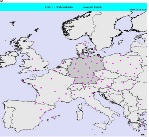
Figure 4.The LINET network , source LINET GMBH, taken from [14]
the Cb (approx. 15-20km), as well as for the geolocation error of the satellite (approx 5km), and for 139
the security distance defined for flying round of a Cb. The study focuses on central Europe where the 140
LINET network density is the highest, see Figure4. The borders of the validation region are as follows: 141
Latitude 45.5-56.5 N and Longitude 2.0-18.0 East. 142
The skill scores Probability Of Detection (POD), False Alarm Rate (FAR), Critical Success Index (CSI) are used to measure the performance of the different approaches. For completeness the quantities are defined below:
POD=CD/(CD+MD) (3)
CSI=CD/(CD+MD+FD) (5) Hereby, CD stands for Correct Detection of a Cb, MD stands for Missed Detection of a CB and FD 143
stands for False Detection and CDN stands for Correct Detection of Nil. The validation is performed 144
on a pixel basis. This means that each pixel is assigned with either CD, FD, MD or CDN. Missed 145
detection is counted if lightning occurs but there is no Cb detected by the satellite within the search 146
radius. 147
Experiments 1-11 have been performed performed for the period 10.05.16-09.06.16, for 6,9,12,15,18 148
UTC respectively. The experiments 12-14 dealing with KO and respective intercomparison experiments, 149
needed to evaluate the KO skill scores, have been performed for June 2017. This has been necessary as 150
KO is not archived for the 2016 period. Both periods are characterized by frequent occurrence of Cbs 151
for different weather situations, seize and structure. 152
Two experiments have been performed using additionally the BT difference of the ozone channel 153
(IR9.7) and the 8.7 channel (9.7-8.7). The IR9.7 channel is the ozone channel and has a clear sky emission 154
peak in the stratosphere see figure2. Thus, it can be assumed that clouds reaching the stratosphere 155
(overshooting tops) show a pronounced signal if the ozone channel is used for the calculation of the 156
BT difference as discussed e.g by [16]. Overshooting tops are a specific feature of Cbs. Thus, the use of 157
the ozone channel might be useful to omit the NWP filter at a certain BT difference (height), which 158
has been investigated in experiment 5 and 6. However, the physical basis is the same as discussed in 159
[5], but with the ozone emission interacting with the cloud emission instead of water vapour/cloud 160
interaction. 161
3.2. Results 162
Tables 1 shows the skill scores of the experiments in detail. Following the main results of the 163
experiments are summarized. 164
The results show that applying a NWP filtering can be used to optimize the relation of POD and 165
FAR and thus, to improve the critical success index. For the experiments with NWP filter a relative 166
high POD in combination with a relative low FAR can be gained, leading to significant better CSI than 167
without NWP filtering. 168
POD is slightly higher without NWP filtering, but FAR is strongly affected towards higher values, 169
leading to a significant decrease of CSI. However, compared to the experiments without NWP filtering 170
higher POD can be achieved, accompanied by better CSI and FAR, by application of the NWP filter 171
and lowering of the BT difference threshold (Experiments 1-4). These results clearly demonstrates 172
that the NWP filter does significantly increases the performance of the satellite based detection of Cbs. 173
Thus, also for applications where a high POD is the primarily goal, and FAR and CSI are of second 174
priority, the NWP filter is of significant benefit. 175
The additional usage of theO3channel does not lead to better skill scores compared to the 176
reference (experiment 1). On the other hand, the one channel approach (experiment 9) leads to similar 177
skill scores compared to the reference (experiment 1). The physical basis of these results is further 178
discussed in section4 179
Experiment 7 and 8 shows the effect of a slight variation of the NWP filter threshold on the 180
skill scores. Finally in experiment 10 and 11 CAPE from ICON has been used instead of CAPE from 181
ECMWF. The results show that the skill scores are not significantly affected by the NWP source for 182
CAPE. Thus, the NWP filtering is not sensitive to the NWP model in our experiments. 183
Further experiments (12-14) for June2017 has been performed with KO from ICON as this stability 184
filter has been recommended by the weather forecast department based on their daily practice. In 185
order to evaluate the skill scores for KO intercomparison experiments for the same period has been 186
performed with CAPE (as the skill scores are not independent on the chosen period). The investigated 187
hours and the region are the same as for 2016. Thus the same number of samples have been used for 188
The results indicate that KO performs similarly to CAPE. In this experiment KO leads to higher 190
POD, but due to also lower FAR the CSI is lower as well. However, the differences are relative small. 191
By consideration of the results given in table Table 1 it is obvious that a higher CSI could be gained 192
with KO by decrease of the KO threshold. The combination of KO and CAPE does not lead to better 193
skill scores than KO alone. 194
The accuracy is close to 100 % for all experiments and is therefore not an appropriate skill score 195
for Cb detection, although, it is sometimes used as score for events with low probability of occurrence. 196
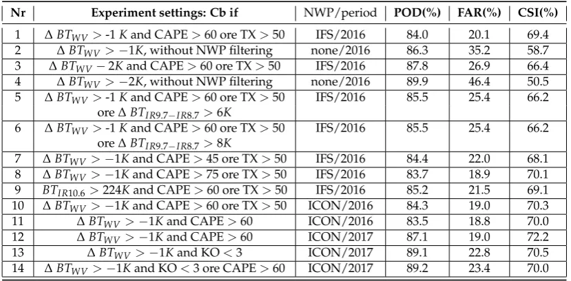
Table 1. Results of the different experiments. ∆means the difference of IR channels, wherebyWV
means that of the the water vapor channels, otherwise the channels are explicitely noted. NWP/period provides the model used for NWP filtering and whether the investigated summer period was in 2016 or 2017. IFS is the forecast model of ECMWF and ICON of DWD. The other columns provide the probability of detection (POD), false alarm rate (FAR) and the critical success index (CSI)
Nr Experiment settings: Cb if NWP/period POD(%) FAR(%) CSI(%)
1 ∆BTWV>-1Kand CAPE>60 ore TX>50 IFS/2016 84.0 20.1 69.4 2 ∆BTWV >−1K, without NWP filtering none/2016 86.3 35.2 58.7 3 ∆BTWV−2Kand CAPE>60 ore TX>50 IFS/2016 87.8 26.9 66.4 4 ∆BTWV >−2K, without NWP filtering none/2016 89.9 46.4 50.5 5 ∆BTWV>-1Kand CAPE>60 ore TX>50 IFS/2016 85.5 25.4 66.2
ore∆BTIR9.7−IR8.7>6K
6 ∆BTWV>-1Kand CAPE>60 ore TX>50 IFS/2016 85.5 25.4 66.2 ore∆BTIR9.7−IR8.7>8K
7 ∆BTWV>−1Kand CAPE>45 ore TX>50 IFS/2016 84.4 22.0 68.1 8 ∆BTWV>−1Kand CAPE>75 ore TX>50 IFS/2016 83.7 18.9 70.1 9 BTIR10.6>224Kand CAPE>60 ore TX>50 IFS/2016 85.2 21.5 69.1 10 ∆BTWV>−1Kand CAPE>60 ore TX>50 ICON/2016 84.3 19.0 70.3 11 ∆BTWV>−1Kand CAPE>60 ICON/2016 83.5 18.8 70.0 12 ∆BTWV>−1Kand CAPE>60 ICON/2017 87.1 19.0 72.2 13 ∆BTWV>−1Kand KO<3 ICON/2017 89.1 22.8 70.5 14 ∆BTWV>−1Kand KO<3 ore CAPE>60 ICON/2017 89.2 23.4 70.0
The application of the NWP filter works well independent which of the two NWP models (ICON 197
or ECMWF) or if CAPE ore KO are used as stability filter. One reason for this finding might be that the 198
NWP parameter are applied as filter to filter stable and neutral atmospheres and are therefore very 199
permeable for satellite based Cb detection as soon as labile atmospheric conditions occurs. 200
4. Discussion 201
The results of our study show that the 1 channel approach works as good as the established BT 202
difference approach and the investigated 4 channel approach. This might be astonishing on a first 203
glance and the physics behind this finding is therefore briefly discussed. 204
The radiation signal from optical thick clouds results from the top of the cloud. Thus, concerning 205
Cbs the satellite observes only the top of the cloud. A long history of publications provide evidence 206
that optical thick clouds can be treated as blackbody. This means that the the Stefan Boltzmann law 207
can be applied for radiances emitted by optical thick clouds. 208
BT defined by the Stefan-Boltzmann law, which results from Planck equation.
R=σ∗T4 (6)
In other wordseλcan be assumed to be 1 in the grey body version of the Stefan-Boltzmann law.
This means that in all channels the information of the cloud target (for optical thick clouds) is 209
equal and results simply from the temperature of the cloud top. Thus, there is no possibility to apply 210
IR spectroscopy and additional channels does not provide additional information about the cloud 211
physical properties or if the cold temperature results from a mature (active) Cb or another type of 212
optical thick cloud. Following a brief review of the respective publications. 213
Stephens [17] compared parameterization schemes with observational data and found thateλ 214
equals 1 for clouds with a liquid water path (LWP) above a 80-120 (g/m2). This finding is independent 215
on the cloud type. Beside Cbs, e.g. also cumulus clouds, nimbostratus clouds and stratocumulus II 216
clouds can easily exceed 120g/m2[17]. Further, for the same LWP the emissivity is quite similar for 217
different cloud types below 80-120 (g/m2), with exception of Stratus II. Please see [18] for a description 218
of the cloud types. 219
Further, he discussed a parameterization of the effective emissivity of clouds, given in equation8
eλ=1−exp(−a0∗W) (8) Hereaois the absorption mass coefficient for total infrared flux (empirically found to be 0.13) and W is
220
the total vertical liquid water path. It is evident that this parameterization leads to aneλof 1 for high 221
W. This parameterization is well established and widely used in different fields. 222
Lio [19] reports that the monochromatic flux emissivityeλis given to a good accuracy by
eλ=1−exp(−D∗a0(λ)∗W) (9) This form of the parameterization, with a D=1.66 is aplied as parameterization of ice clouds for 223
climate models [20]. The reader should note that averaging over wavelength is usually necessary in 224
global models for practical reasons. Nevertheless the form remains the same. 225
Also [21] applied a similar parameterization as [17] for the study of cumulus clouds, but uses the optical depth instead of the LWP path. Equation8transforms therefore to
eλ =1−exp(−0.75∗τc) (10)
here,τcis the total cloud optical depth. A similar equation, but with an factor of -0.5 instead of -0.75, is
226
applied for radiance fitting within the scope of Remote Sensing of cloud top pressure/height from 227
SEVIRI [3]. Both, approaches lead to a emissivity of 1 for optically thick clouds. 228
[22] compared a fast radiative transfer model (RTM) with DISORT [23] and found for the 229
8.5-,11-,12-µmwavelength that the brightness temperature difference between the models decrease to 230
negligible values with increasing optical depth of ice clouds. This means that optical thick (opaque) ice 231
clouds behave like blackbodies within the uncertainties of the RTMs. This result is in accordance with 232
the above mentioned RTM parameterizations. 233
[24] uses the blackbody feature of Cbs as basis for the determination of the Effective Emissivity 234
of semitransparent cirrus clouds by bi-spectral measurements based on AVHRR channels 4 and 5 235
(10.3-11.3µmand 11,5 - 12,5µm). [25] uses the same approach for with GMS-1 data. 236
[26] investigated the long-wave optical properties of water clouds and rain with Mie scattering 237
theory for the wavelength region 5-200µm. They found that for the long-wave radiation (IR) the cloud 238
becomes a black-body for large LWP (large means greater than 100). 239
Finally, [27] discussed physics principles in radiometric infrared imaging of clouds in the 240
atmosphere. He investigated also IR emissivity by application of the RTM MODTRAN [28] . His 241
results confirms that the emissivity of optically thick clouds is 1, and that they emit a nearly ideal 242
blackbody spectrum. 243
Summarizing, clouds with large optical thickness behave as blackbodies in the IR SEVIRI channels. 244
By consideration of the uncertainty of the radiance measurements and calibration uncertainties of the 245
the temperature of the cloud top for optical thick clouds. Thus, a MSG multiple channel approach does 247
not provide information if the cold cloud is a active Cb or another optical thick cloud. Thus, they can 248
not be used to reduce the FAR of the satellite based detection of Cbs. Contrarily, this can be done by 249
application of the NWP filter as demonstrated in section3 250
Using the water vapour brightness temperature difference eases the visible inspection of images 251
and is beneficial for the application of optical flow, applied for the short term forecast of Cbs. However, 252
similar skill scores can be achieved with a 1 channel approach. 253
Finally, it might be reasonable to clarify why different BT differences occurs (equivalent to different 254
RGB images) if different channels are used, see for example figure 2 in [16]. For the WV channels, as 255
well as for the ozone and CO2 channel the atmospheric signal received by the satellite results from a 256
mixture of the radiation emitted by clouds and from of emission by water vapor, ozone or CO2 for the 257
WV, ozone and CO2 channels, respectively. This interaction leads to different BT signals depending on 258
the chosen channels for the calculation of the BT differences. Thus, this leads to a different relation 259
between the observed brightness temperatures and the cloud top height. 260
5. Materials and Methods 261
For the forecast runs ECMWF operational model [12] at 00h and 12h has been used. This means 262
that forecasts up to 9 hours are applied. For comparison ICON [13] has been used. In contrast to 263
ECMWF ICON forecast runs are applied every 3 hours. Thus, the respective run 3 hours prior relative 264
to the satellite scanning time has been used. 265
The satellite Brightness temperature are derived from the level 1.5 rectified image data of digital 266
counts by application of the Eumetsat calibration coefficients and conversation method. More detailed 267
information on MSG and the SEVIRI instrument are given [29]. 268
The lightning data and the applied methods are discussed in detail in section3and section2, 269
respectively. 270
6. Conclusions 271
The performed experiments shows that the satellite based detection of Cbs can be significantly 272
improved by application of an appropriate NWP stability filter. The application of NWP filtering leads 273
to a large decrease of FAR and a large increase of CSI, demonstrating the performance of the filter to 274
separate Cb clouds from other optical thick clouds. The decrease of POD, resulting from the NWP 275
filtering, can be compensated by a reduction of the BT threshold. Thus, NWP filtering can be used 276
to optimize the relation between POD and FAR and to improve the detection scores. Hence, also for 277
applications where a high POD is the primarily goal, and FAR is of second priority, the NWP filter is of 278
vital importance. We show that KO index as well as CAPE are appropriate NWP stability filter. Further 279
more, using ECMWF or ICON forecasts as source for stability filters lead to a similar performance 280
in our experiments. Optical thick clouds behave as black bodies. IR spectroscopy can therefore not 281
be applied in order to decide if a cold optical thick cloud is a active Cb or another cloud type. Thus, 282
a multiple channel approach can not replace the function of NWP filtering. As a result of the study 283
DWD implemented the method based on the brightness temperature difference with a threshold of -1 284
Kelvin and KO as NWP stability filter as operational Cb detection method for aviation. 285
Acknowledgments:We thank the weather forecast team of DWD, in particular Mr. Koppert, Mr. Barsleben and
286
Mr. Diehl for the discussion and advice concerning the development of the Cb detection method, in particular 287
concerning the selection of the NWP stability parameters. 288
Author Contributions:Richard Mueller developed the method and performed the validation study supported
289
by Stephane Haussler. Matthias Jerg initialised and managed the project and contributed to the writing of the 290
manuscript. 291
Conflicts of Interest:The authors declare no conflict of interest
Abbreviations 293
The following abbreviations are used in this manuscript: 294
295
ACC Accuracy or hit rate BT Brightness Temperature
Cb Cumulonimbus
CSI Critical Success Index CTH Cloud Top Height
ECMWF European Centre for Medium Weather forecast. FAR False Alarm Rate
ICON NWP model of Deutscher Wetterdienst KO Convection Indec
MSG Meteosat Second Generation Meteosat Meteorological satellite NWP Numerical Weather Prediction POD Probability of Detection
SEVIRI Spinning enhanced visible and infrared imager 296
References 297
1. Gijben, M.; Coning, C. Using Satellite and Lightning Data to Track Rapidly Developing Thunderstorms in 298
Data Sparse Regions. Atmospher2017,8. 299
2. Donovan, M.F.; Williams, E.R.; Kessinger, C.; Blackburn, G.; Herzegh, P.H.; Bankert, R.L.; Miller, S.; F., 300
M. The Identification and VErificantion of Hazardous Convective Cells over Oceans Using Visible and 301
Infrared Satellite Observations. Journal of Applied Meteorology and Climatology2008,47. 302
3. Hamann, U.; Walther, A.; Baum, B.; Bennartz, R.; Bugliaro, L.; Derrien, M.; Francis, P.N.; Heidinger, A.; Joro, 303
S.; Kniffka, A.; Le Gléau, H.; Lockhoff, M.; Lutz, H.J.; Meirink, J.F.; Minnis, P.; Palikonda, R.; Roebeling, 304
R.; Thoss, A.; Platnick, S.; Watts, P.; Wind, G. Remote sensing of cloud top pressure/height from SEVIRI: 305
analysis of ten current retrieval algorithms. Atmospheric Measurement Techniques2014,7, 2839–2867. 306
4. Mosher, F. Detection of deep convection around the globe. Preprints, 10th Conf. on Aviation, Range, and 307
Aerospace Me- teorology. American Meteorological Society, 2002, pp. 289–292. Portland. 308
5. Schmetz, J.; Tjemkes, A.; Gube, M.; van der Berg, L. Monitoring deep convection and convective 309
overshooting with Meteosat. Advances in Space Research1997,19, 433–441. 310
6. Autones, F. Algorithm Theoretical Basis Document for Rapid Development Thunderstorms. Technical 311
report, NWC-SAF, 2013. 312
7. Tag, P.M.; Bankert, L.R.; Brosy, L.R. An AVHRR multiple cloud-type classification package. Journal of
313
Applided Meteorology2000,39, 125–134. 314
8. Berendes, T.A.; Mecikalski, J.R.; Mackenzie, W.M.J.; Bedka, K.M.; Nair, U.S. Convective cloud identification 315
and classification in daytime satellite imagery using standard de- viation limited adaptive clustering. 316
Journal of Geophsical Research2008,113. 317
9. Zinner, T.; Forster, C.; de Coning, E.; Betz, H.D. Validation of the Meteosat storm detection and nowcasting 318
system Cb-TRAM with lightning network data – Europe and South Africa. Atmospheric Measurements
319
Techniques2013,6, 1567–1583. 320
10. Moncrief, M.W.; Miller, M.J. The dynamics and simulation of tropical cumulonimbus and squall lines.Q. J.
321
R. Meteorol. Soc.1976,120, 373–394. 322
11. www.ecmwf.int/en/forecasts/documentation-and-support/changes-ecmwf-model/ifs-documentation. 323
last visit 10.09.2017. 324
12. Bechtold, P.; Köhler, M.; Jung, T.; Doblas-Reyes, F.; Leutbecher, M.; Rodwell, M.J.; Vitart, F.; Balsamo, 325
G. Advances in simulating atmospheric variability with the ECMWF model: From synoptic to decadal 326
time-scales. Quarterly Journal of the Royal Meteorological Society2008,134, 1337–1351. 327
13. Zängl, G.; Reinert, D.; Rípodas, P.; Baldauf, M. The ICON (ICOsahedral Non-hydrostatic) modelling 328
framework of DWD and MPI-M: Description of the non-hydrostatic dynamical core. Quarterly Journal of
329
14. Betz, H.D.; Schmidt, K.; Laroche, P.; Blanchet, P.; Oettinger, W.P.; Defer, E.; Dziewit, Z.; Konarski, J. LINET 331
— An international lightning detection network in Europe. Atmospheric Research2009,91, 564 – 573. 332
15. Betz, H.; Schmidt, K.; Oettinger, W.; Montag, B. Cell-tracking with lightning data from LINET.Advances in
333
Geoscience2008,17, 55–61. 334
16. Mikuš, P.; Mahovi´c, N.S. Satellite-based overshooting top detection methods and an analysis of correlated 335
weather conditions. Atmospheric Research2013,123, 268–280. 336
17. Stephens, G. Radiation Profiles in Extended Water Clouds II: Parameterization Schemes. J. Atmos. Sci.
337
1978,35, 2123–2132. 338
18. Stephens, G. Radiation Profiles in Extended Water Clouds I: Theory. J. Atmos. Sci.1978,35, 2111–2122. 339
19. Liou, K.Radiation and cloud processes in the atmosphere; Oxford University Press, 1992. 340
20. Ebert, E.E.; Curry, J.A. A Parameterization of Ice Cloud Optical Properties for Climate Models. Journal of
341
Geophysical Research1992,97, 3831–3836. 342
21. Xu, K.M.; Randall, D.A. Impcat of Interactive Radiative Transfer on the Macroscopic Behaviour of Cumulus 343
Ensembles. Part I: Radiation Parameterization and Sensitivity Tests.Journal of the Atmospheric Sciences1995, 344
52, 785–799. 345
22. Wang, C.; Yang, P.; Baum, B.A.; Platnick, S.; Heidinger, A.K.; Hu, Y.; Holz, R.E. Retrieval of Ice Cloud 346
Optical Thickness and Effective Particle Size Using a Fast Infrared Radiative Transfer Model. Journal of
347
Applied Meteorology and Climatology2011,50, 2283–2297. 348
23. Spurr, R.; Kurosu, T. A Linearized Discrete Ordinate Radiative Transfer Model for Atmospheric Remote 349
Sensing Retrieval.J. Quant. Spec. Radiat. Trans.2001,68, 689–735. 350
24. Inoue, T. On the Temperature and Effective Emissivity Determination of Semi-Transparent Cirrus Clouds 351
by Bi-Spectral Measurements in the 10µmwindow region. Journal of the Meteorological Society of Japan1985, 352
63, 88–99. 353
25. Nasuda, H. Infrared Greybody Emissivity and Visible Albedo of High Altitude Semitransparent Cloud.?
354
1985.
355
26. Savijäri, H.; Räisänen, P. Long-wave optical properties of water clouds and rain. Tellus1998,50A, 1–11. 356
27. Shaw, J.A.; Nugent, P.W. Physics principles in radiometric infrared imaging of clouds in the atmosphere. 357
European Journal of Physics2013,34. 358
28. Abreu, L.; Anderson, G. The MODTRAN 2/3 Report and LOWTRAN 7 MODEL. Technical report, Philips 359
Laboratory, Hanscom, 1996. 360
29. Schmetz, J.; Pili, Tjemkes, P.S.; Just, D.; Kerkmann, J.; Rota, S.; Ratier, A. An introduction to Meteosat 361