Classification Of PEC Detect Using Hybrid
Technique
V.Leelavathy [1], Dr.J.Komalalakshmi [2]
1 Research Scholar, SNR Sons College, Coimbatore
2 Assistant Professor, Department of Computer Science,SNR Sons College, Coimbatore
Abstract--- In aircraft fuselage, multilayer structures are used mostly and detect the defect in this structure by using eddy current testing. Compared to conventional eddy current pulse excitation eddy current is most important. These methods are used for flaw detection and defect characteristics. Lift off effect and interlayer air gaps are main thing in eddy current defect characteristics. In this work proposed a hybrid approach to predict or reduce this defect using genetic algorithm with Library support vector machine. In this work three phases are implemented that are feature extraction, normalization and classification. In feature extraction dimensionally reduction are done by using Independent component analysis and classification are handled by hybrid approach of Genetic algorithm with Library Support Vector Machine (GA-LIBSVM). From the result observed that the proposed method proves the better accuracy of 96.66 compared to existing method of SVM as 90.32. The proposed framework used the data from GMR data theory.
I. INTRODUCTION
Data mining is a recently emerging field, connecting the three worlds of Databases, Artificial Intelligence and Statistics. The information age has enabled many organizations to gather large volumes of data. However, the usefulness of this data is negligible if “meaningful information” or “knowledge” cannot be extracted from it. Data mining, otherwise known as knowledge discovery, attempts to answer this need. In contrast to standard statistical methods, data mining techniques search for interesting information without demanding a priori hypotheses. As a field, it has introduced new concepts and algorithms such as association rule learning. It has also applied known machine-learning algorithms such as inductive-rule learning (e.g., by decision trees) to the setting where very large databases are involved. Data mining techniques are used in business and research and are becoming more and more popular with time.
Eddy currents are generated when time varying magnetic fields are applied to conducting materials satisfying Faraday’s law [1]. These currents flow in such a way that secondary magnetic fields are produced to oppose the applied (primary) magnetic field satisfying Lenz’s law [1]. Pulsed eddy currents (PEC) have favorable advantages over conventional eddy currents (CEC). They are a result to the sum of a continuum of odd number harmonics of the fundamental sinusoidal waveform frequency of the pulse [3, 4]. Therefore, a transient response obtained from the pulsed eddy current system contains many frequencies. Because of the skin effect [5, 6], the depth to which eddy currents penetrate the tested specimen depends on the frequency of applied field in CEC. However, skin effect depends on the duty cycle period of the probing pulse in PEC [5]. Therefore using PEC allows the inspection of various specimen depths with just one pulse as opposed to the multiple frequency scans required for CEC.
Pulsed eddy current (PEC) testing employs pulses as excitation so that the greater amount of frequencies in a response is able to reflect richer information at many depths
[7]. Based on analysis of the response waveform in the time domain, the lift-off intersection point where the transient signal is insensitive to variations in the lift-off height can be selected to suppress lift-off effects [8, 9], but the lift-off intersection point greatly relies on the probe’s structure and specimen’s conductivity, which may weaken the probe’s generality. More effects will be implemented on post processing. With the goal of decreasing the lift-off effect, time frequency domain analysis [10] was also proposed to separate the lift-off effect from influence caused by metal loss and interlayer gap variations.
II. RELATED WORK
In eddy current applications, the distance between the pick-up coil and the specimen is referred to as lift-off. Variations in this parameter tend to affect the time delay to the peak of the received signal in the reference subtracted signal [11]. A crossing point for varying steps of lift-off with all other parameters kept constant was first observed by Waidelich and Haung [12]
Giguere et al [13] and Lefebvre et al [14] have reported on the successful use of the crossing point phenomenon in eliminating lift-off effects in PEC evaluation of conducting specimen. They were able to extract the thickness of a material independent of lift-off by time gating the signals around the time of the lift-off point of intersection. Safizadeh et al [15] however observed that the crossing point actually varied and they considered other aspects of the signal to separate effects due to lift-off and thickness.
III. METHODOLOGY
In propose system current pulse eddy current defect classification is very much useful for aircraft. The two main properties of pulse eddy current are lift – off effect and interlayer air gaps. In proposed work, Independent component analysis (ICA) and hybrid method of Genetic algorithm with Library SVM (LibSVM) are investigated for defect automated classification under different interlayer gaps and lift-off effects.
Figure 1: Block Diagram for Proposed System
ICA
Normalization
Classification using GA with LibSVM
Input
Output
Data’s are collected from the GMR dataset. Then the data’s are dimensionally reduced using Independent Component Analysis (ICA) method then it is normalized and given into classification using hybrid method of Genetic algorithm (GA) with Library Support Vector Method (LibSVM).
A. Independent component analysis
Several ICA algorithms have been proposed so far, which are different in objective functions (or contrast functions) for statistical independence and how to derive ICA algorithms [16, 17 and 18].
REFERENCES
In general, estimated independent components obtained by using these algorithms are different each other. However, it is difficult to discuss which algorithms are most appropriate for feature extraction of characters in the present circumstances. Hence, in the followings, we shall adopt Fast ICA algorithm proposed by Hyvarinen and Oja [19] from its convergence speed.
Suppose that we observe a m-dimensional zero mean input
signal at time t, v(t) = v , … . , v ′ where ‘ means the
transposition of matrices and vectors. Then the n-dimensional whitening signal, x (t), is given by the following equation:
x(t) = Mv(t) = D ⁄ E′v(t) (1)
Where M means a n × m(n ≤ m) whitening matrix that is
given by a matrix of eigenvalues, D, and a matrix of eigenvectors, E. Here, assume that v (t) is composed of n statistically independent signals, s(t) = s (t), … . , s (t) ′ . Then, the following linear transformation from x(t) to s(t) exists:
s(t) = Wx(t) (2) W = w , … , w , is often called a separating matrix, and it
can be acquired through the training of a two-layer feed forward neural network. This neural network has n outputs denoted as s(t) = s (t), … . , s (t) ′ and the ith row vector,
w′(i = 1, … , n), ofW corresponds to a weight vector from
inputs to the ith output s.
The term 'independent' is used here according to the following definition in statistics:
p s (t), … . , s (t) = ∏ pi s (t) (3)
Where p . is a probability density function. Since the
above probability density function is not preliminary unknown, suitable objective functions should be devised such that neural outputs, s are satisfied with Eq. (3) as much as possible, that
s(t) ≈ s(t). Karhunen and Oja have proposed the following objective function [10], J(.), to be maximized in terms of output signals S:
J(s) = ∑ E s~ − 3 E s` (4)
Where E{.} means expectation. As well known, Eq.(4)
corresponds to the fourth-order cumulants of s (t) called
kurtosis. Learning algorithms for a separation matrix, W, are derived from the gradient of Eq. (4). In the followings, we adopt Fast ICA algorithm proposed by Hyvarinen & Oja in which fixed points of the gradient are obtained on-line.
B. Normalization:
Since the quantities of the feature vector may be quite different, a normalization process is required to standardize all the features to the same level. Normalizing the standard deviation and mean of data permits the network to treat each input as equally essential over its range of values. We have
used the function ‘mapstd’ to normalize the inputs and
targets so that they will have zero mean and unity standard deviation.
C. Classification using Hybrid Method:
Classification is done by using Genetic algorithm with Library Support Vector Machine.
i. Genetic algorithm:
The genetic algorithm is a well-known meta-heuristic algorithm, following the natural evolution processes. Haupt and Haupt [20] stated that like any other meta-heuristic algorithm, GAs do not guarantee to find the optimal solution.
Figure 2: Block Diagram for Genetic Algorithm
Algorithm for Independent Component Analysis Pseudo-code for estimating the independent components S of the original data X, and for decomposing X in terms of the estimated components S.
Step 1: X = X − X
Step 2: ∑ × = VΛV
Step 3: R × = √Λ V
Step 4: Y = RX , cov(Y ) = I
Step 5: Apply the ICA code to estimate the p
independent components S × and the corresponding
mixing matrix B × such that Y = BS
Step 6: X = R Y = R BS
Step 7: X = X + X = R BS + X = AS +
X where A × = R B
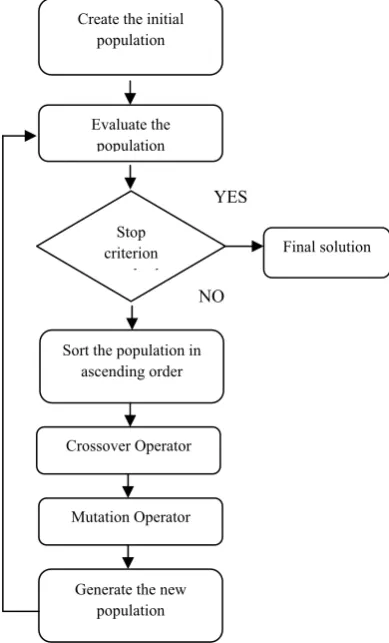
Create the initial population
Evaluate the population
Stop criterion
h d
Sort the population in ascending order
Crossover Operator
Mutation Operator
Generate the new population
Final solution
YES
The GAs commence by defining optimization variables, objective functions, and control parameters [21]. Usually, GAs receive works on an initial population involving the individual solutions represented by ‘‘chromosomes’’, which are strings include all the genes (i.e. variables) involved in a possible solution. The chromosomes are evaluated based on the ‘‘objective function’’, which is the desired objective of the problem
In any iteration of the GA, some of the current individuals are replaced with new generated offspring. ‘‘Crossover rate’’ is defined as ratio of the number of offspring produced in any iteration to the population size. A pair of individuals from the current population is selected as the parents of a pair of offspring. Highly fitted individuals, relative to the whole population, have a higher chance to be selected as parents in next generation, while less fitted individuals have a correspondingly low probability of being selected [22].
GAs are good at taking larger, potentially huge, search spaces and navigating them looking for optimal combinations of things and solutions which we might not find in a life time. GAs is very different from most of the traditional optimization methods. Genetic algorithms need design space to be converted into genetic space. So, Genetic algorithms work with a coding of variables. The advantage of working with a coding of
variable space is that coding discretizes the search space even though the function may be continuous. A more striking difference between GAs and most of the traditional optimization method is that GA uses a population of points at one time in contrast to the single point approach by traditional optimization methods. This means that GA processes a number of designs at the same time
ii. Library Support Vector Machine (LIBSVM)
The figure 2 illustrates the flowchart for proposed framework. LIBSVM is a library for Support Vector Machines (SVMs). The goal is to easily apply SVM to their applications. LIBSVM has gained wide popularity in machine learning and many other areas. In this work, we present implementation of LIBSVM. Issues such as solving SVM optimization problems theoretical convergence multiclass classification probability estimates and parameter selection. A typical use of LIBSVM involves two steps: first, training a data set to obtain a model and second, using the model to predict information of a testing data set. For SVC and SVR, LIBSVM can also output probability estimates.
This is same as SVM technique; where in training SVM the m by 1 vector of training labels (type must be double) is taken.
STEP 1: [Start] Generate random population of n chromosomes
STEP 2: [Fitness] Evaluate the fitness f(X) of each chromosome X in the population
STEP 3: [NEW population] Create a new population by repeating following steps until the new population is complete.
[Selection] Select two parent chromosomes from a population according to their fitness
[Crossover] with a crossover probability, cross over the parents to form new offspring (children). If no crossover was performed, offspring is the exact copy of parents.
[Mutation] with the mutation probability, mutate new offspring at each locus
STEP 4: [REPLACE] Use new generated population for a further run of the algorithm
STEP 5: [Test] If the end condition is satisfied, stop, and return the best solution in current population
STEP 6: [Loop] GO to step 2
Figure 3: Flow Chart for Proposed Work
Select one off-spring
Apply Mutation operator to produce Mutated offspring
Assign fitness to off-springs Mutation
Finished
Natural Selection
Mutation No
Apply replacement operator to incorporate new individual into population
Terminate? No
Yes
Start
Seed Population Generate N individuals
Assign fitness to each individual
Select two individuals (Parent 1 Parent 2
Use crossover operator to product off-springs
Assign fitness to off-springs Crossover
finished No Natural
Selection
Reproduction Recombination
Natural Selection
Yes
LIBSVM (Training, Testing, Command)
Alpha, Cost specifications are come under the
command
IV. EXPERIMENTAL RESULT
In this section, the artificial defects in two-layer specimen with various interlayer air gaps and lift-offs are automated classified with the proposed method. The experimental results are evaluated using MATLB. The proposed method of ICA with LIBSVM is compared with the existing method of PCA with SVM.
Figure 4: Schematic of two-layer specimen.
The specimen can provide four sets of defects:1st-layer surface defects and1st-layer sub-surface defects shown in Figure 4 (a), 2nd-layer surface defects and 2nd-layer sub-surface defects in Figure 4 (b)., the distance l between the probe and specimen is used to simulate the various lift-offs is shown in figure 4 (c). Distance d between two plates in Figure 4 (d) is used to simulate the inter layer air gaps
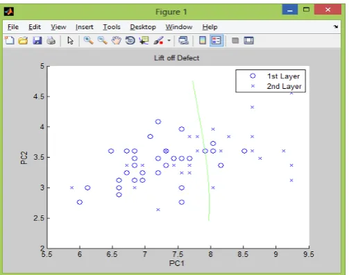
Figure 5: Classification results of 1st-layer surface and 2nd layer for lift-offs
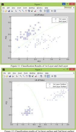
Figure 6: Classification results of 1st-layer surface and 2nd layer surface
Figure 7: Classification results of 1st-layer and 2nd layer subsurface
Figure 9: Classification results of 1st-layer and 2nd layer surface
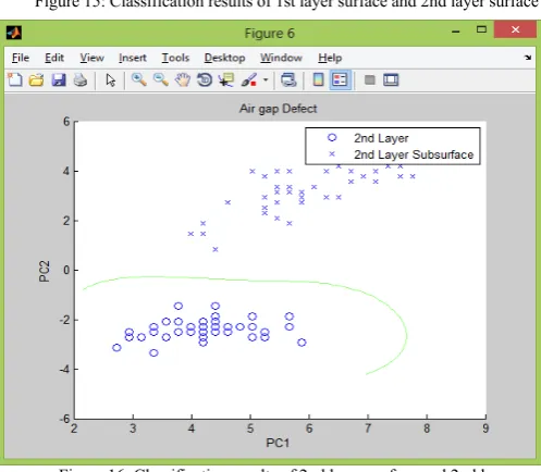
Figure 10: Classification results of 2nd layer and 2nd layer subsurface
The figure 5 illustrates the classification result of 1st layer and 2nd layer for lift-off. The defects in two-layer specimen with various lift-offs and the constant air gap are classified. Figure 6 shows the classification result of 1st layer and 2nd layer surface for lift-off. Figure 7 gives the classification result of 1st layer and 2nd layer subsurface for lift-off defect. The differential time responses DT of all defects are used to generate the new features through the conventional PCA-based method and the first two PCs are used to classify the defects through the SVM-based method. Figure 8 shows the classification results of 1st-layer and 2nd-layer defects. Figure 9 shows the classification results of 1st-layer surface and 2nd-layer surface. Figure 10 illustrates the shows the classification results of 2nd layer surface and 2nd-layer subsurface.
To overcome these and prove better accuracy by proposed system of ICA with LIBSVM.
Figure 11: Classification Results of 1st Layer and 2nd Layer
Figure 12: Classification results of 1st layer surface and 2nd layer surface
Figure 14: Classification results of 1st layer surface and 2nd layer
Figure 15: Classification results of 1st layer surface and 2nd layer surface
Figure 16: Classification results of 2nd layer surface and 2nd layer subsurface
The figure 11 illustrates the classification results of 1st layer and 2nd layer for defection lift-offs of proposed method of ICA is used for dimensionally reduction and the classification is obtained by using GA-LIBSVM. Figure 12 illustrates the classification results of 1st layer surface and 2nd layer surface for defection lift-offs. Figure 13 illustrates the classification results of 2nd layer surface and 2nd layer surface for defection lift-offs. Figure 14 illustrates the classification results of 1st layer surface and 2nd layer for air gap defection. Figure 15 illustrates the classification results of 1st layer surface and 2nd layer surface for air gap defection. Figure 16 illustrates the classification results of 1st layer surface and 2nd layer subsurface for air gap defection.
Figure 17: Comparison of Accuracy
Figure 18: Comparison of Time
The figure 17 and 18 illustrates the comparison of accuracy and time between the proposed methods of ICA with GA_LIBSVM. From the figure clearly observes that the proposed method proves the better result than the existing method. That the proposed method gives the accuracy of 96.66% with 984.53s and the existing method provides the accuracy of 90.32% with 6.8s.
TABLE I COMPARISON BETWEEN EXISTING AND PROPOSED SYSTEM
SPECIMEN EXISTING PROPOSED ACCURACY PARAMETER
SPECIFICATION
The specimen can provide four set of defects: 1st layer surface defects, 1st layer
sub surface defects, 2nd layer surface defects and 2nd
layer sub-surfaces defects
Existing methods are done by using
Principal component Analysis (PCA)
with Support Vector Machine
(SVM). Defect classification with
various air gaps and air liftoffs
Proposed methods are done by using
Independent component Analysis (ICA) with Genetic Algorithm library Support Vector Machine (LIBSVM). Defect classification with various air gaps and
air liftoffs.
By Comparing both two defects accuracy can be calculated. A measure of a
predictive model that reflects the proportionate
number of times that the model is correct when
applied to data. Accuracy is calculated
from the equation Accuracy
= TN + TP
TN + FP + FN + TP Where TN is the number of true negative cases
FP is the number of false positive cases
FN is the number of false negative cases
TP is the number of true positive cases
It specifies the algorithm used for proposed and existing for lift off and air gap.
With liftoff the defects can be
classified
The defects in two layer specimens with various liftoffs
from 0mm to 1.4 mm and the air gap 0mm are classified
The defects in two layer specimens with various liftoffs
from 0mm to 1.4 mm and the air gap 0mm are classified.
With air gap the defects can be
classified
The interlayer gaps d in two-layer specimen vary from 0mm to 1.4mm and
the liftoff l is constant at 0mm.
The interlayer gaps d in two-layer specimen vary from 0mm to 1.4mm and
the liftoff l is constant at 0mm. For liftoff
1) 1st layer
2ND
LAYER
The defect in two layer specimen with various lift off and the constant air gap are classified.
The classification results of 1st layer and 2nd layer for defection lift-offs of proposed method
of ICA is used for dimensionally reduction and the
classification is obtained by using
GA-LSVM
Existing Proposed Existing Proposed
Accuracy is calculated from the above equation for PCA with SVM Accuracy is calculated from the above equation for ICA with GA-LIBSVM PCA with SVM ICA with LIBSVM
2) 2nd layer 2nd layer sub
surface
The defect in two layer specimen with various lift-offs and constant
air gap are classified. The results are obtained
using PCA and
The classification results of 2nd layer
and 2nd layer sub surface for detection lift-offs proposed method of
ICA is used for dimensionally
SPECIMEN EXISTING PROPOSED ACCURACY PARAMETER SPECIFICATION
SVM. This defect is much better than
previous defect
reduction and the classification is obtained by using GA-LIBSVM. The
accuracy is much better than the existing method Accuracy is calculated from the above equation for PCA with SVM Accuracy is calculated from the above equation for ICA with GA-LIBSVM PCA with SVM ICA with LIBSVM
For air gap
1st layer
2nd layer
The differential time responses DT
of all defects are used to generate the
new features through the conventional PCA based method and the first two PCs are used to classify the defects through the SVM based
method
The classification results of 1st layer and 2nd layer for air gap defection of proposed method of ICA is used for
dimensionally reduction and the
classification is obtained by using GA-LIBSVM. The
accuracy is much better than the existing method
Existing Proposed Existing Proposed
Accuracy is calculated from the above equation for PCA with SVM Accuracy is calculated from the above equation for ICA with GA-LIBSVM PCA with SVM ICA with LIBSVM
2nd layer surface
2nd layer surface
The differential time responses DT
of all defects are used to generate the
new features through the conventional PCA based method and the first two PCs are used to classify the defects through the SVM based
method
The classification results of 1st layer and 2nd layer for air gap defection of proposed method of ICA is used for
dimensionally reduction and the
classification is obtained by using GA-LIBSVM. The
accuracy is much better than the existing method.
Existing Proposed Existing Proposed
Accuracy is calculated from the above equation for PCA with SVM Accuracy is calculated from the above equation for ICA with GA-LIBSVM PCA with SVM ICA with LIBSVM Overall maximum values for both Existing and Proposed for Accuracy and
Time
The maximum values of defects air
gap and liftoff with PCA and LIBSVM
are denoted in accuracy and time
The maximum values of defects air
gap and liftoff with ICA and GA-LIBSVM are denoted in accuracy
and time. Overall Existing Accuracy Overall proposed Accuracy Overall existing time Overall proposed time
Table 1 provides the overall comparison between the existing and proposed system. From the comparison table clearly observed that the proposed system provides the better result.
Table II COMPARISON OF ACCURACY AND TIME FOR EXISTING LIFT OFF
LAYERS ACCURACY TIME(s)
1st layer
2nd layer 83.33 4
1st layer surface
2nd layer surface 90 4
2nd layer surface
2nd layer sub surface. 90 3
Table III COMPARISON OF ACCURACY AND TIME FOR EXISTING AIR GAP
Layers Accuracy Time
1st layer
2nd layer 90 3
1st layer surface
2nd layer surface 90 4
2nd layer surface
2nd layer sub surface. 93.33 3
Table IVCOMPARISON OF ACCURACY AND TIME FOR PROPOSED LIFTOFF
Table V COMPARISON OF ACCURACY AND TIME FOR PROPOSED AIR GAP
Table VICOMPARISON OF ACCURACY FOR LIFT OFF BEFORE NORMALIZATION
Table VIICOMPARISON OF ACCURACY FOR AIR GAP BEFORE NORMALIZATION
Table 1 to 7 provides the comparison table for proposed and existing accuracy and time for lift off and air gap and results obtained before normalization.
LAYERS ACCURACY TIME
1st layer
2nd layer 90 15
1st layer surface
2nd layer surface 93.33 18
2nd layer surface 2nd layer sub
surface.
96.66 15
LAYERS ACCURACY TIME(s)
1st layer
2nd layer 93.33 10
1st layer surface
2nd layer surface 96.66 12
2nd layer surface
2nd layer sub surface. 96.66 12
LAYERS Existing Proposed
1st layer
2nd layer 80 83.33
1st layer surface
2nd layer surface 76.66 80
2nd layer surface
2nd layer sub surface. 80 836.66
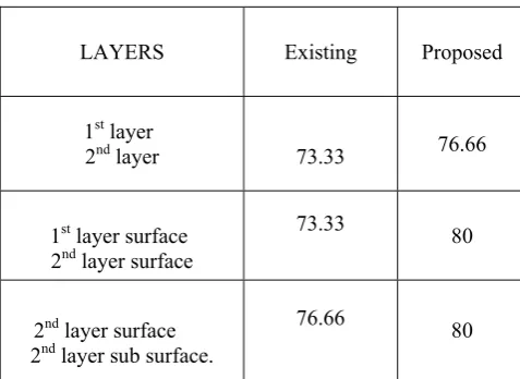
LAYERS Existing Proposed
1st layer
2nd layer 73.33 76.66
1st layer surface 2nd layer surface
73.33 80
2nd layer surface 2nd layer sub surface.
Figure 18: Comparison of Accuracy for lift off for all layers.
.
Figure 19: Comparison of Accuracy for Air Gap for all layers.
Figure 20: Comparison of layers depth
Figure 21: Comparison of Amplitude for layers
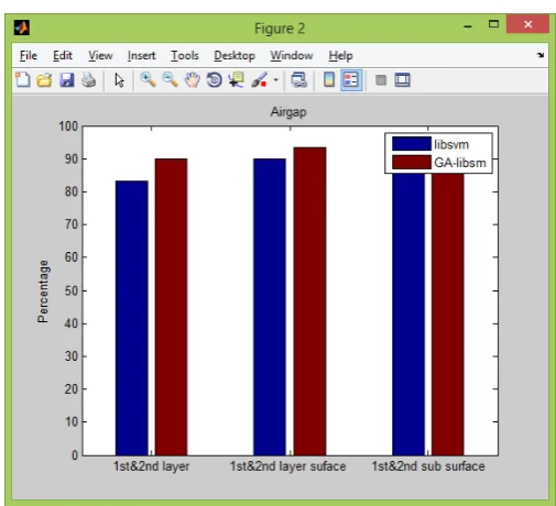
Figure 18 illustrates the accuracy for lift off of all the layers between LIBSVM and Genetic Algorithm with LIBSVM. From the figure clearly observed that the combination of GA with LIBSVM provides the better result. Figure 19 illustrates the accuracy for Air Gap of all the layers between LIBSVM and Genetic Algorithm with LIBSVM. From the figure clearly observed that the combination of GA with LIBSVM provides the better result. Fi9gure 20 and 21 illustrates the comparison of layers and their amplitudes.
V. CONCLUSION
In this work, defect automated classification in aircraft multiply structure is investigated through pulsed eddy current with the help of ICA and GA-LIBSVM. Defects in two-layer. The PEC technique with the help of ICA and GA-LIBSVM can build the model for defect automated classification in two-layer structures. The defects on different layers can be classified satisfactorily using the proposed method.
This hybrid approach is very useful and accurately defect the lift-off and air gaps. In Genetic Algorithm, three steps are followed that are selection, crossover and mutation. In mutation part that pbest and gbest are produced and it is given to the command of alpha and cost specification of LIBSVM. From the experiment result proves that the proposed method classify best and give accuracy as a better one than existing one.
REFERENCES
[1] R. A. Serway and J. W. Jewett. Physics for scientists and Engineers, with modern physics, pages 967–1002. Thomson Brooks/Cole, New York, USA, 6th edition, 2000.
[2] N. Mohan, T. M. Undeland, and W. P. Robbins. Power
Electronics, Converters, Applications and Designs. John Wiley and Sons, Inc, New York, USA, 2nd edition, 1995.
[3] E. Kreyszig. Advanced Engineering Mathematics, pages
431–485. Wiley International Edition, New York, USA, second edition, 1967.
[4] C. Tia, J. H. Rose, and J. C. Moulder. Thickness and
conductivity of metallic layers from pulsed eddy current measurements. Review of scientific Instruments, 67(11):3965–3972, November 1996.
[5] A. Krawcyzyk and J. A. Tegopoulos. Numerical Modelling of Eddy Currents, pages 1–42. Clarendon Press-oxford, 1993.
[6] A. Sophian, G.Y. Tian, D. Taylor, J. Rudlin, Design of a
pulsed eddy current sensorfor detection of defects in aircraft lap-joints, Sensors and Actuators A: Physical101 (2002) 92–98
[7] Grossinger, R., Kupferlinga, M., Kasperkovitz, P., et al.,
Eddy Currents in Pulsed Field Measurements, J. Magn. Magn. Mater., 2002, vol. 242, pp. 911–914.
[8] Giguere, S., Dubois JMS. Pulsed Eddy Current: Finding
Corrosion Independently of Transducer Lift-Off, Rev. Prog. Quant. Nondestr. Eval. , 2001, vol. 19, pp. 49–56.
[9] Giguee, S., Lephine, B.A., and Dubois, J.M.S., Pulsed
Eddy Current Technology: Characterizing Material Loss with Gap and Lift-Off Variations, Res. Nondestruct. Eval. , 2001, vol. 13, pp. 119–129.
[10] Safizadeh, M.S., Lepine, B.A., Forsyth, D.S., and Fahr,
A., Time Frequency Analysis of Pulsed Eddy Current Signals, J. Nondestruct. Eval. , 2001, vol. 22, pp. 73–86.
[11] D. L. Waidelich. Pulsed Eddy Currents. ‘Research
Techniques in Non-destructive Testing, Academic press’, pages 383–416, 1970.
[12] D. L. Waidelech and C. R. Lahmeyer. The testing of thick
sheets of metal using Pulsed Eddy Currents. Technical report, University of Missouri Colombia, Missouri 65211, USA, 1979.
[13] J. R. S. Giguere and J. M. S. Dubios. Pulsed Eddy
Current: Finding corrosion independently of transducer lift-off. Review of progress in QNDE, 19:449–456, 2002.
[14] J. H. V. Lefebvre and J. M. S. Dubois. Lift-off Point of
Intercept (LOI) Behaviour. 31st Review of progress in QNDE, 17, Summer 2001.
[15] M. S. Safizadeh, B. A. Lepine, D. S. Forsyth, and A. Fahr. Time frequency analysis of pulsed Eddy Current signals. Journal of Nondestructive Evaluation, 20(2):73–87, June 2001.
[16] Lambers, H and Poorter, H. “Inherent variation in growth
rate between higher plants: A search for physiological causes and ecological consequences. Advances in Ecological Research 23, 187-261.
[17] Corn leaf analysis and interpretative Guidelines, Olsen’s
Agricultural Laboratory, Inc, 2008.
[18] J. A. Silva and R. Uchida, “Essential Nutrients for Plant
Growth: Nutrient Functions and Deficiency Symptoms”, College of Tropical Agriculture and Human Resources, University of Hawaii at Manoa, 2000.
[19] A. Hyvarinen and E. Oja “A fast fixed-point algorithm for
independent component analysis", Neural Computation, 9, 1483-1492, 1997.
[20] R.L. Haupt, S.E. Haupt, Practical Genetic Algorithms,
John Wiley and Sons Inc., New Jersey, 2004.
[21] A. Sokolov, D. Whitley, Unbiased tournament selection,
in: The Conference on Genetic and Evolutionary Computation, GECCO’05, ACM, Washington DC, 2005, pp. 1131–1138.
[22] S. Sivanandam, S. Deepa, Introduction to Genetic