Development of a Computational Method for Assessing Static Field Induced Torque on Medical Implants

Scholarship@Western

Scholarship@Western

Electronic Thesis and Dissertation Repository

8-26-2019 2:00 PM

Development of a Computational Method for Assessing Static

Development of a Computational Method for Assessing Static

Field Induced Torque on Medical Implants

Field Induced Torque on Medical Implants

Xiao Fan Ding

The University of Western Ontario Supervisor

Chronik, Blaine A.

The University of Western Ontario

Graduate Program in Medical Biophysics

A thesis submitted in partial fulfillment of the requirements for the degree in Master of Science © Xiao Fan Ding 2019

Follow this and additional works at: https://ir.lib.uwo.ca/etd

Part of the Medical Biophysics Commons

Recommended Citation Recommended Citation

Ding, Xiao Fan, "Development of a Computational Method for Assessing Static Field Induced Torque on Medical Implants" (2019). Electronic Thesis and Dissertation Repository. 6452.

https://ir.lib.uwo.ca/etd/6452

This Dissertation/Thesis is brought to you for free and open access by Scholarship@Western. It has been accepted for inclusion in Electronic Thesis and Dissertation Repository by an authorized administrator of

Abstract

The objective of this thesis is the development of a computational method for finding the torque induced on an object when placed in the static magnetic field of an MR scanner. As a preliminary step, the classic EM problems of a sphere and infinitely long cylinder of linear material was modeled in commercially available simulation software. Upon verification of the parameters implemented, the second step is the simulation of simple objects with realistic material properties, stainless-steel cylinders. Physical cylinders were machined to match those in the simulations and underwent the ASTM standard method for measuring induced torque. An adjacent study that was also performed was finding the measurement uncertainty in a prototype ASTM abiding apparatus, separate from the one used for experimental verification.

It was found that the sphere and infinitely long cylinder models differed less than 5% from the analytical solutions. Implementing the correct material properties, magnetic susceptibility in particular, to the grades of stainless-steel used in this study was particularly challenging. However, when the experimentally measured results were used to find the necessary susceptibility values for the computational methods, it was found to be in agreement with literature values. The following computationally-found torque values agreed within 10% difference from the experimentally measured values. The induced torque increased linearly with the length of the cylinders and the square of magnetic susceptibility.

In the uncertainty analysis of the torque measurement apparatus described in ASTM F2213-17, it was found that the apparatus described in the ‘Pulley Method’ offered a lower instrument uncertainty than the apparatus described in the ‘Torsional Spring Method’. This study emphasized on the contribution of static friction and is important to consider should the apparatus be used in the future to verify computational results.

Summary for Lay Audience

Magnetic Resonance Imaging (MRI) is a method of visualizing the inside of the human body by using a variety of magnets to create a complex electromagnetic environment, or MR environment, contained within the scanning room. Since the 1990s, MRI has seen widespread adoption around the world and has since received a reputation being a safe imaging method due, in part, to the intense scrutiny that MRI technicians place on what is allowed into the scanning room.

A common signage at any MRI site is the warning that ‘The Magnet is Always On’. When foreign material, anything not already contributing to the MR environment, enter the MRI site, it may interact with the magnetic fields being generated. Material of any kind have magnetic properties. Pure iron for example, can fly across the scanning room, like a projectile, due to the displacement force exerted on it by the scanner’s magnetic fields. Human tissue, on the other hand, is so weakly magnetic that they appear to be inert until extremely high magnetic field strengths, far above what is currently clinically approved.

Co-Authorship Statement

It is the intention of the author to publish the work presented in Chapter 2 co-authored by Xiao Fan Ding, William B. Handler, and Blaine A. Chronik. William Handler offered assistance and suggestions in to the development of the computational methods used as well as data analysis. William Handler and Blaine Chronik reviewed the written work. Blaine Chronik aided in apparatus setup and taking measurements for validation of simulations and was responsible for overall supervision of the study. Development of the computational methods, production of scripts, measurements, analysis, and writing was performed by Xiao Fan Ding.

The work presented in Chapter 3 was submitted and accepted as an abstract to the international Society of Magnetic Resonance in Medicine (ISMRM) 1. This body of work was presented as a digital poster at ISMRM 2019 and it is the intention of the author to publish this work co-authored by Xiao Fan Ding, William B. Handler, and Blaine A. Chronik. William Handler offered assistance and suggestions on improvements in the data analysis. William Handler and Blaine Chronik reviewed the written work. Blaine Chronik was responsible for overall supervision. Apparatus setup, measurements, writing, and analysis was performed by Xiao Fan Ding.

1 _{Ding, X., Handler, W. B., & Chronik, B. A. (2018). UncertaintyAnalysis of Torque}

Acknowledgements

The work presented in this thesis could not have been completed without all those who have offered their guidance and support in my personal and professional development. I would like to use this space to give my acknowledgements to those people.

First and foremost, I must thank Dr. Blaine Chronik who has acted as my supervisor for the past two years. He gave me the opportunity to work at the xMR Labs and guided me through the trials and tribulations of academic research. In addition, I would like to acknowledge Dr. William Handler, the lead researcher at the xMR Labs and an indispensable source of knowledge through his intelligence, wit, and humour. Our interactions were few but each one worthwhile. I would also like to acknowledge my advisory committee, Dr. Tamie Poepping and Dr. Jean Theberge and The Ontario Research Fund, NSERC, and Canadian Foundation for Innovation as sources of funding.

Furthermore, I would like to acknowledge Frank van Sas, Brian Dalrymple, and Derek Gignac for the design and manufacturing of the apparatuses used throughout my research as well as machining of the stainless-steel rods. Not to mention, occasionally they would 3D print Star Wars figurines that I designed on a whim.

My experience with graduate school got off to a rough start. When at my lowest, I could always count on my lab mates to raise my spirits. On my first day I was in the company of Christopher Brown, Amgad Louka, Eric Lessard, Kieffer Davieau, and Arjama Halder. Along the way Diego Martinez and John Adams joined our group. I know without a doubt that I will forever cherish the friendships I’ve made in the past two years.

Table of Contents

Abstract ... ii

Summary for Lay Audience ... iii

Co-Authorship Statement ... iv

Acknowledgements ... v

Table of Contents ... vi

List of Figures and Tables ... x

List of Symbols and Abbreviations ... xii

Chapter 1: Introduction

1.1 Motivation ... 2

1.2 Research Objective ... 4

1.3 MR Systems ... 4

1.3.1 The Main Magnet ... 8

1.3.2 The Gradient Coils ... 11

1.3.3 The Radiofrequency Coils ... 14

1.3.4 The Electromagnetic Environment of an MRI System ... 17

1.3.5 The Screening Process for Patients Entering the MR Environment ... 19

1.4 Medical Devices ... 22

1.4.1 Electromagnetic Material Properties ... 24

1.4.2 Interactions with an MR Scanner ... 26

1.4.2.1 Radiofrequency Interactions ... 27

1.4.2.2 Gradient Interactions ... 29

1.4.2.3 Magnetically Induced Displacement Force ... 31

1.4.2.4 Magnetically Induced Torque ... 33

1.5 Electromagnetic Interactions Relevant to Torque ... 35

1.5.1 A Sphere of Linear Magnetic Material ... 36

1.5.2 An Infinitely Long Cylinder of Linear Magnetic Material ... 38

1.5.3 Force and Torque on a Magnetic Dipole Moment ... 39

1.6 Regulatory Environment ... 39

1.6.1 How Large Families of Implants Are Assessed ... 41

1.6.2 ASTM Methods for Device Interactions in MR ... 42

1.6.3 ASTM Methods for Torque Assessment ... 43

1.7 Thesis Overview ... 47

Chapter 2: Computational Evaluation of Stainless-Steel Cylinders

for Static Field Induced Torque

2.1 Introduction ... 55

2.2 Theory ... 56

2.2.1 Magnetic Field Inside and Outside of a Sphere ... 59

2.2.2 Magnetic Field Inside and Outside of an Infinitely Long Cylinder ... 59

2.2.3 The Force on a Magnetic Dipole Moment ... 60

2.2.4 The Volume Magnetic Susceptibility of Stainless-Steel Alloys ... 60

2.3 Methods ... 63

2.3.1 Part 1: Verification of Parameters for Simulating Linear Magnetic Material in a Static Magnetic Field ... 63

2.3.2 Part 2: Simulation of Stainless-Steel Rods in a Static and Uniform Magnetic Field... 66

2.3.2.1 Computational Setup ... 67

2.3.2.2 Experimental Setup ... 70

2.4 Results ... 75

2.4.1 Part 1: 3D Slice Plots from COMSOL and Analytical Plots MATLAB …... 75

2.4.2 Part 1: Verification with Analytical Solution ... 78

2.4.3 Part 2: Finding the Magnetic Susceptibilities of the Stainless-Steel Cylinders 80 2.4.4 Part 2: Experimentally Measured Induced Torque ... 82

2.5 Conclusion... 84

2.5.1 Validity of Using FEM to Find the Field Inside and Outside of Objects of Linear Magnetic Material ... 84

2.5.2 Verification of Computational Method to Calculate the Torque Induced on Stainless-Steel Cylinders from the Static Field of an MR Scanner ... 84

Chapter 3: Uncertainty Analysis of Torque Measurement Methods

Described in ASTM F2213-17

3.1 Introduction ... 89

3.2 Theory ... 90

3.2.1 Error Propagation in the Torsional Spring Method ... 90

3.2.2 Error Propagation in the Pulley Method ... 91

3.2.3 Sources of Measurement Uncertainty... 92

3.3 Methods ... 93

3.4 Results ... 96

3.5 Conclusion ... 99

3.6 References ... 100

Chapter 4: Thesis Summary, Future Directions, and Conclusion

4.1.1 Chapter 2 Summary ... 101

4.1.2 Chapter 3 Summary ... 102

4.2 Future Directions ... 102

4.1.1 Investigate Torque Induced on Better Characterized Material ... 102

4.1.2 Extend Computational Torque and Force Models to More Complex Objects 102 4.1.3 Investigate Eddy Current Torque ... 103

4.1.4 Automating Computational Processes ... 103

4.1.5 Investigate Very Long Objects Experiencing Interactions in Tandem ... 104

4.1.6 Extend Uncertainty Analysis of Rotating Test Platforms ... 104

Appendix A: Derivation of Equations

A.1 Spherical and cylindrical coordinates ... 107

A.2 Finding the magnetic flux density inside and outside of a sphere of linear material with the external field along z-direction ... 108

A.3 Finding the magnetic flux density inside and outside of an infinitely long cylinder of linear material with the external field perpendicular to the cylinder ... 111

A.4 Finding the static field induced torque on a sphere ... 113

Appendix B: Certificate of Tests for Stainless Steel Rods

B.1 Stainless steel 316 rod, diameter of 0.5 in. and length of 1 ft. ... 115

B.2 Stainless steel 316 rod, diameter of 0.25 in. and length of 1 ft. ... 117

B.3 Stainless steel 304 rod, diameter of 0.5 in. and length of 1 ft. ... 119

B.4 Stainless steel 304 rod, diameter of 0.25 in. and length of 1 ft. ... 121

Appendix C: Calibration Reports for Laboratory Equipment

C.1 MR03-025 Force Sensor (Mark-10 Co., Copiague, USA) ... 123

C.2 SPX123 Laboratory Balance (Ohaus Co., Parsippany, USA) ... 124

Appendix D: Permission to Use Copyrighted Figures

D.1 Allen D. Elster of MRIquestions.com ... 126

D.2 Standards Council of Canada Letter of Agreement ... 127

D.3 John Wiley and Sons License Terms and Conditions ... 129

D.4 ASTM International License Terms and Conditions ... 133

D.5 Cambridge University Press License Cover Sheet ... 139

List of Figures and Tables

Figure Page

1.3-1 The components of an MR system ... 6

1.3-2 Cross-sectional view of an MR system ... 7

1.3-3 Applying shims to the main magnet ... 10

1.3-4 Main magnet coil windings and active shielding ... 10

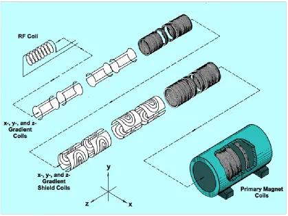
1.3-5 Positioning of RF, gradient, and main magnet coils ... 13

1.3-6 Trapezoidal gradient pulse shape ... 14

1.3-7 Birdcage and surface coils ... 16

1.3-8 Saddle and birdcage coil designs ... 17

1.3-9 The MR environment within 5 Gauss ... 19

1.3-10 ACR zoning recommendation for MR suites ... 21

1.4-1 ASTM symbols for MR safe, unsafe, and conditional ... 23

1.4-2 Spectrum of magnetic susceptibility ... 26

1.4-3 Device interactions from static, gradient, and RF fields ... 27

1.4-4 Schematic of the deflection test method for static field induced force ... 32

2-1 Orientation of the external magnetic field ... 58

2-2 Sphere and cylinder models in COMSOL ... 64

2-3 Meshed sphere and cylinder models in COMSOL ... 65

2-4 Set of cylinders in COMSOL ... 68

2-5 Positions of 3 cm long cylinder exported from COMSOL ... 70

2-6 Crank operated linear displacement mechanism ... 71

2-7 Machined stainless-steel cylinders ... 72

2-8 Rotating apparatus holding cylinders ... 73

2-9 Measurement setup in the MR suite ... 74

2-10 Magnetic flux plots from COMSOL ... 76

2-11 Magnetic flux plots based on analytical solution ... 77

2-12 Analysis of field inside and outside of sphere ... 78

2-13 Analysis of field inside and outside of cylinder ... 79

3-1 Schematic diagram of apparatus from ASTM F2213-17 ... 94

3-2 Schematic and photograph of apparatus designed for the pulley method ... 95

3-3 Propagation of errors for the ‘Torsional Spring’ and ‘Pulley’ methods ... 98

A-1 Spherical and cylindrical coordinates ... 107

Table Page 2-1 Magnetic susceptibility values for stainless-steel alloys ... 61

2-2 ASTM composition requirements for SS304 and SS316 ... 62

2-3 Equations for susceptibility curves ... 81

2-4 Measured peak torque values ... 82

2-5 Comparison of measured and simulated peak torque values ... 83

3-1 ‘Break torque’ observations ... 97

List of Symbols and Abbreviations

MR and MRI Magnetic resonance and magnetic resonance imaging CADTH Canadian Agency for Drugs and Technologies in Health OECD Organization for Economic Co-operation and Development ICDs Implantable cardioverter defibrillators

RF Radiofrequency

PNS Peripheral nerve stimulation

FDA Food and Drug Administration

NbTi Niobium-titanium

LHe Liquid helium

SNR Signal-to-noise ratio

DSV Diameter of spherical volume

𝐁 and 𝐁𝟎 Magnetic flux density (‘B-field’) and external magnetic flux _density 𝐇 and 𝐇_𝟎 Magnetic field strength (‘H-field’) and external magnetic field

strength

EMF Electromotive force

NMR Nuclear magnetic resonance

𝜔₀ Larmor frequency

𝛾 Gyromagnetic ratio

𝐌 Magnetization

SAR Specific absorption rate

ACR American College of Radiology

ISO International Organization for Standardization

ASTM ASTM International (formerly ‘American Society for Testing and Materials’)

CDRH Center for Devices and Radiological Health 𝜇_𝑚 or 𝜇 Permeability of the material

𝜇0 Permeability of vacuum

𝜇_𝑟 Relative permeability

𝜒_𝑚 or 𝜒 Volume magnetic susceptibility AIMDs Active implanted medical devices

EPI Echoplanar imaging

𝐅_𝐦 Magnetically induced displacement force

𝐦 Magnetic dipole moment

𝑀𝑠 Saturation magnetization

𝑉 and 𝑑𝑉 Volume of device and volume of element

DUT Device under testing

𝜃 Deflection angle

𝐅𝐠 Weight (‘force due to gravity’)

𝜌 Density

𝐠 Acceleration due to gravity

𝑁_𝑛 and 𝑁_𝑡 Demagnetizing factor perpendicular to the plane of the device and demagnetizing factor in the plane of the device

𝑊𝑇 Magneto-static energy per unit volume

𝛼 Angle of the saturation magnetization with respect to the normal in plane of the device

𝑅 Radius

𝛕 Torque

PMA Premarket approval

NEMA National Electrical Manufacturers Association 𝐹 and 𝐹𝑓 Force and frictional force

𝐿 Longest dimension of device

𝜇 Coefficient of friction

𝜃_repose Angle of repose

𝑘 Torsional spring constant

∆𝜃 Deflection angle in torsional spring method

FEM Finite element method

SS 304 and SS 316 Stainless-steel grade 304 and 305

mfnc Magnetic fields, no currents

PDE Partial differential equations

Chapter 1

Introduction

1.1 Motivation

Magnetic Resonance Imaging (MRI) is a non-invasive and non-ionizing imaging modality that has seen annual growth in Canada and abroad. In Canada, three times as many MRI units were installed than decommissioned between 2012 and 2016, suggesting a trend of net growth in the future [2]. An estimated 1.86 million MRI examinations were performed in the 2017 to 2018 Canadian fiscal year, approximately 51 examinations per 1000 people, up from 1 million MR scans in 2007 [1]. Internationally, the Organization for Economic Co-operation and Development (OECD), an intergovernmental economic organization whose mission is to improve the economic and social well-being of people around the world, uses the number of MRI units and examinations as a metric for assessing quality of healthcare [3]. Amongst OECD members, there was an upwards trend in the number of MRI examinations between 1995 to 2017 [4].

The growth in the use of MRI has been in parallel with the growth in the implementation of permanent and semi-permanent implantable medical devices [5]. In 2003, over 370,000 implants of device-based therapies using implantable cardiac systems, pacemakers and implantable cardioverter defibrillators (ICDs), occurred in the United States [5]. In Canada, there were more than 120,000 patients and 15,000 patients living with pacemakers and ICDs respectively [6]. With the growth of these two phenomena, it is estimated that 50-75% of patients living with such an implant will require an MRI exam over the lifetime of their device [5].

There have been no indications that fields as high as 16 T have an adverse effect on animal subjects, well above the 1.5 T to 3 T fields used in clinical scanners [7,8]. In 2017, the FDA approved the first clinical 7 T scanner limited to the head and extremities, arms and legs [55]. Although exposure to strong magnetic fields have not shown adverse effects on patients without medical implants, the same cannot be said for patients with medical implants.

As mentioned, up to 75% of patients living with medical implants may require an MR exam over the lifetime of their device however, there are concerns regarding safety when examining patients with medical implants. These concerns include, but are not limited to, magnetically induced displacement force and torque, gradient and RF induced heating, and gradient induced vibrations [9,10,11]. It becomes clear that the growth of MRI as a diagnostic tool together with the increased use of medical implants, there is a need to accurately and systematically test for the safety of such devices in the MR environment.

Commercially available medical implants need to be approved by a governing body to enter an MR scanner. To determine the risk that an implant poses, implants are subjected to experimental testing outlined by test standards for different interactions between implant and scanner. Test standards are available for investigating the following, but are not limited to, force torque from the static field, heating, vibrations, and voltages from the pulsed gradient coils, and heating from the RF coils [11,13-15]. The results from testing for each interaction are compiled to create a safety label that stipulate whether an implant is safe, unsafe, or conditional in an MR scanner [26]. This thesis focuses on magnetically induced torque.

Therefore, it includes the uniform field inside the scanner, the static field gradient around the scanner, the pulsed gradients and RF fields as well.

1.2 Research Objective

The objective of this thesis was to design simulations capable of accurately determining the magnetically induced torque on entire families of medical implants in the MR environment. As previously mentioned, there are other possible interactions between the implant and the MR environment, those interactions are not discussed in this thesis. A simulation may alleviate the workload of assessing the safety of all the commercially available medical implants. Provided the static magnetic field along with the material, geometry, and orientation of the device being tested, the simulations should have the capacity to output the induced torque for any combination of the aforementioned parameters. The simulations are not intended to replace physical testing altogether, but rather, to go through the many configurations that exist and identify the ‘worst-case’ configurations. The identified worst-case configuration is then subjected to physical testing to identify the conditions for which it is safe for the implant to be present in the MR scanner.

1.3 MR Systems

Permanent Magnets – The magnetic field of a permanent magnet is always present. Unlike current-driven magnets, permanent magnets supply a magnetic field for an indefinite amount of time with no cost to maintenance [17,19]. A common material used to produce permanent magnets is an alloy of aluminum, nickel, and cobalt known as alnico [16]. The use of permanent magnets is limited due to being extremely heavy and a maximum static field of less than 1 T [50].

Resistive Magnets – These are made up of coils of wire through which and electrical current is passed [17]. The field strength of resistive magnets is dependent on the current that passes through the coils. Resistive magnets are less limited by weight than permanent magnets but require much higher costs due to the large quantities of power required to maintain the magnetic field [16]. The maximum field strength of a system made from resistive magnets is typically 0.6 T due to its excessive power requirements [16,17].

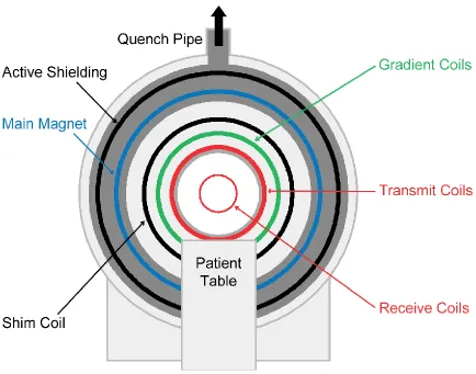
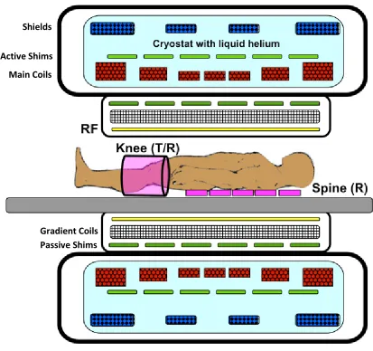
Figure 1.3-2: A cross-sectional view of an MRI scanner. The most exterior object is the main magnet which houses the main magnet coils (red), active shims (green), and active shielding (red) all submerged in liquid helium. Nested within the main magnet are gradient coils (b/w grid) and a set of passive shims (green). An RF transmit/receive coil (pink, left) is placed over the knees of the patient and a set of receive only coil array (pink, right) are placed below the spine. Courtesy of Allen D. Elster, MRIquestions.com.

Active Shims

Main Coils Shields

1.3.1 The Main Magnet

The main magnet supplies the static magnetic field, 𝐁_𝟎. This field is in the direction of the bore, where the patient lies. Low-field MRI magnets (less than 0.35 T) use a combination of resistive and permanent magnets. However, resistive magnets require large power consumption and permanent magnets have high installation cost [41]. Over time, low-field scanners have been replaced by 1.5 T scanners while studies that require greater resolution in MRI have been conducted using 7 T and 9.4 T [8,40,41]. The benefit of higher fields is the increased signal-to-noise ratio (SNR), a crucial aspect for image quality. Fields greater than 0.35 T require superconducting magnets, with 1.5 T scanners being the predominant field strength in the clinical setting, MRI is the largest commercial application of superconductivity [41].

In theory, superconducting magnets require no power to maintain once a current is established since zero electrical resistance means the current never dies out. In reality, imperfections in coil design add some resistance to the circuit and over time, there is a loss in magnetic field. Historically, the LHe used to supercool coil windings regularly evaporates into gas that needs to be expelled into the atmosphere requiring refills every 4.5 months [17,41,42]. Modern magnets have zero-boil off technology allowing helium gas to re-condense into LHe within the cryostat [41,42].

Ideally, the region of the scanner bore where the patient lies should have a completely homogeneous static field from the main magnet. Field homogeneity is measured in parts per million (ppm) over a certain diameter of spherical volume (DSV). The magnetic isocenter is the centre of the DSV. The requirement for commercial 1.5 T and 3 T magnets is a homogeneity on the order of 10 ppm of the static field over a 50 cm DSV [41]. For context, any two positions within ± 25 cm of the magnetic isocentre of the bore should not differ more than 1.5 µT or 3 µT on a 1.5 T or 3 T scanner respectively. The loss in field strength should be no more than 0.1 ppm per hour [41,42].

passive and active shimming. In the absence of a patient, passive shimming is performed by placing ferromagnetic metal sheets, shims, in shim trays that are arranged along the circumference of the bore [41,43]. When field inhomogeneities arise from interactions between a patient and the static field, active shimming is used. Shim coils, either superconducting or resistive magnets, rely on a current to generate a magnetic field opposite to the inhomogeneities [17].

A quench refers to the loss of superconductivity, and consequentially the magnetic field, when the coil windings are raised above the critical temperature [17]. NbTi is superconducting at approximately 10 K and cooled in LHe at 4.7 K [17,39]. During a quench, the heat generated raises the temperature enough such that there is a large amount of boil-off of LHe [17]. The quench pipes are to guide the gas out of the building. Quenches can be accidental or intentional in emergencies, such as when there is a fire in the scanner room or when a patient is pinned to the scanner. The latter is a concern when ferromagnetic objects in the scanner room become a projectiles due to an induced force from the static field. In those events, the field needs to be turned off by an emergency quench [51].

Figure 1.3-3: a) Diagram showing the arrangement of shim trays (yellow) along the inner bore of the magnet (blue). b) Photograph of shim trays arranged along the magnet bore. c) Positioning the shim tray. Courtesy of Allen D. Elster, MRIquestions.com.

1.3.2 The Gradient Coils

The purpose of the gradient magnetic fields from the gradient coils is to spatially encode the positions of the nuclei of the sample in the scanner by creating a variation in the Larmor frequency, the intrinsic processional frequency of a magnetic dipole in an external magnetic field, as a function of position [36,49]. The cylindrical gradient coils are placed inside the bore and sit between the main magnet and the RF coils. The most common configuration used consists of three sets of coils used to generate three orthogonal fields 𝐺_𝑥, 𝐺_𝑦, and 𝐺_𝑧 that are pulsed intermittently [35,36]. The role of the gradient coils is to vary the z component of the static field, 𝐵_𝑧, linearly along the Cartesian axes x, y, and z.

The gradients are resistive magnets and the fields are produced by passing a current through the wires arranged on a cylindrical surface. For clinical scanners the gradient strengths are on the order of mT per metre.

The variation in static magnetic field is achieved by superimposing the gradient fields on the static field [16,35]. Since the static field is in the direction of the bore, 𝐵_𝑥 and 𝐵_𝑦 are negligible and assumed to be zero. After the gradients have been applied, the field is still in the direction of the bore, but the field strength varies linearly along x, y, and z depending on the applied gradient. Before applying gradients, the static field is given the following,

Afterwards,

The gradient fields are not always present, they are pulsed intermittently and the rate at which they are pulsed have an operational limit that is in part determined by PNS

𝐺_𝑥 =𝜕𝐵𝑧 𝜕𝑥 𝐺𝑦 = 𝜕𝐵𝑧 𝜕𝑦 𝐺𝑧 = 𝜕𝐵𝑧 𝜕𝑧 (1.3-1) 𝐁 = ( 𝐵_𝑥 𝐵𝑦 𝐵𝑧 ) = ( 0 0 𝐵₀ ) (1.3-2) 𝐁 = ( 0 0

𝐵0+ 𝐺𝑥𝑥 + 𝐺𝑦𝑦 + 𝐺𝑧𝑧

[36]. PNS is discussed in greater detail in section 1.4.2.2 on gradient interactions. In short, by Faraday’s law of induction, a changing magnetic field will induce an electromotive force (EMF), measured in volts, across a conducting material [17,23]. The switching of the gradients can induce a voltage on nerves, conductive tissue in the human body [17]. The effect of stimulation occurs when the induced current exceeds the depolarization threshold of the nerve and initiates an action potential across the cell membrane [17,54].

As mentioned, the gradient fields are pulsed intermittently. By Faraday’s law of induction, the rate of change of pulsed gradients can induce localized electric currents, eddy currents, in conductive material. Scanner components such as the shims, coils, cryostat, and scanner housing are all subject to induced eddy currents. One method to avoid or reduce eddy currents outside the imaging region is to use active shielding. This is accomplished by implanting an additional set of coils, shield coils, that are placed exterior to the gradient coils [36]. The wires of the shield coils are positioned such that the fields generated in between the gradient and shield coils cancel out [36,38].

Figure 1.3-6: A gradient pulse in a trapezoidal shape. Moving from left to right, the strength of the gradient rises from zero to its max amplitude and maintains that amplitude for some time before falling to zero. The reverse then occurs, where the gradient strength falls to the min amplitude and rises to zero. Take for example, when the z-gradient is applied with a max amplitude of 10 mT/m (1 G/cm). Inside of a 120 cm long bore of a 3 T scanner, the field strength along z would vary from 2.994 T to 3 T at the isocentre and to 3.006 T. At the min amplitude of -10 mT/m, the field inside varies from 3.006 T to 2.994 T from end to end. The gradient then rises to zero. The rise and fall times in this figure are equal [16,17].

1.3.3 The Radiofrequency Coils

The physical phenomenon that MRI relies on to generate a signal from is nuclear magnetic resonance (NMR) [17]. NMR describes how nuclei aligned to an external magnetic field are exposed to an RF source at the resonant frequency, it will respond by producing a detectable electromagnetic signal [53]. The application of an RF source that exploits the phenomenon of resonance is termed excitation. In MRI, the nuclei that is often excited is hydrogen, whose nucleus consists of a single proton. The Larmor frequency, 𝜔₀, is an intrinsic property of nuclei with odd number of protons and neutrons. The Larmor

G

frequency is the frequency at which such a nuclear system precesses about an external magnetic field, 𝐁_𝟎, and is directly proportional to 𝐁_𝟎by the gyromagnetic ratio [49].

Excitation of the nuclei and detection of the signal produced is performed by the RF coils. The RF transmit coil send out short bursts of electromagnetic waves in the radio frequency range, known as an RF pulse, to excite the nuclei and the signal produced is detected by the RF receiver coil [16].

In the absence of an external field, the nuclear magnetic moments of the nuclei in a sample are aligned randomly resulting in no net magnetization, 𝐌 [16]. Classically, magnetization is described as net magnetic dipole in a volume [48]. The main magnet supplies the necessary external field, 𝐁_𝟎 , and subsequently generating some net magnetization aligned with 𝐁𝟎. Net magnetization, as with any other vector, can be

separated into components. The longitudinal component, 𝐌_𝐳, is aligned with 𝐁_𝟎 while the transverse component, 𝐌_𝐱𝐲, is in the plane formed by the remaining two directions [49]. With the use of gradients in addition to a strategically chosen and simultaneously applied RF pulse, a particular slab of material can be excited [16,47]. The 𝐌_𝐱𝐲created by resonance can then be detected by a receiver coil [16].

The RF transmit coil produce a time varying RF field, denoted by 𝐁_𝟏, that is perpendicular to 𝐁_𝟎. The net magnetization, 𝐌, is aligned with 𝐁_𝟎 until 𝐁_𝟏is applied at the Larmor frequency and ‘tips’ 𝐌 away by some tip angle, 𝛼. The duration of the applied 𝐁𝟏

field is short and typically in the millisecond range. It is for that reason that they are referred to as RF pulses. After excitation, the signal produced in response to the RF pulse are detected by a receiver coil [17]. To put it simply, it is known that by Ampere’s law, a magnetic field is generated when a current passes through a wire [23]. Conversely, by Faraday’s law, if a loop of wire is exposed to an oscillating field, a current is induced in the loop and the resulting voltage constitutes the MR signal [16,23]. The purpose of the receiver coil is to maximize signal detection while minimizing the noise, in other words, maximize SNR [17].

A volume coil can both transmit and receive and encompasses the entire anatomy for head, extremity, or whole-body imaging [16]. In horizontal bore MR systems, where 𝐁_𝟎is oriented horizontally, the transmit coil is likely to be a saddle coil or birdcage coil design. In a saddle coil, six wires are arranged at 60° intervals. This is so that an approximate sinusoidally varying current around the surface can be achieved. The birdcage coil design improves homogeneity over the saddle coil by increasing the number of conductors. It consists of two conductive loops connected by an even number of conductive rungs [17]. Birdcage coils are capable of yielding uniform SNR over the entire imaging volume [16]. However, although volume coils provide greater uniformity in RF excitation, their large size produce images with lower SNR than other types of coils.

Surface coils tend to be receive-only and are used to improve SNR when imaging structures near the surface of the patient. In general, the closer the coil is to the structure under examination, the greater the SNR as the coil is closer to the signal emitting anatomy. There is also the benefit of shaping surface coils to fit easily near the anatomy since the loop is not restricted to a circle. However, the signal and noise received from surface coils only correspond to volume of area located around the coil. For a circular coil, the depth to which the coils can detect signal is proportional to the radius of the loop [16]. For example, a 10 cm diameter circular loop can image tissue up to 10 cm in length and to a depth of 5 cm. A coil array system uses multiple surface coils whose individual signals are combined to create one image with improved SNR and increased field of view. A drawbacks of surface coils is that smaller loops provide greater SNR at the cost of field of view. Array systems seek to benefit from greater sensitivity to signal and increased coverage.

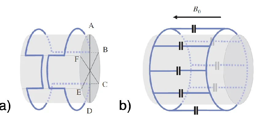
Figure 1.3-8: The saddle coil and birdcage coil designs of transmit/receive volume coils. a) Saddle coil where the current runs from point A to B and so forth until point F. To approximate for a sinusoidally varying current, the conductors at A and D carry zero current while it rises from . b) Birdcage coil consisting of two conductive loops connected by conductive rungs [17]. Reprinted with permission from Cambridge University Press, reference 17.

1.3.4 The Electromagnetic Environment of an MRI System

When biological material such as human tissue is exposed to the MR environment, there are two potentially harmful effects that may occur. The first is heating in tissue due to exposure to RF pulses. The rate of change of the temperature is directly proportional to a quantity known as the specific absorption rate (SAR) which quantifies the power deposited into a mass of tissue by RF exposure and is measured in watts per kilogram. As a precaution, RF tissue heating is restricted to less than a single degree Celsius of the approved SAR limit by body area [9,17]. The second is PNS from the switched gradients [17,37]. Generally, PNS causes discomfort but is not harmful as modern scanners have stimulation monitor that alerts the operator/technician of the likelihood of PNS. It becomes hazardous when occurring on cardiac muscles however, cardiac stimulation requires 80 times the PNS threshold [17]. Extended exposure to the static field however, has shown no long-term adverse biological effects [6,17]. No biological effects have been observed in human subjects under 2 T while there have been reports of fatigue, headaches, and irritability on subjects exposed to fields greater than 2 T [16].

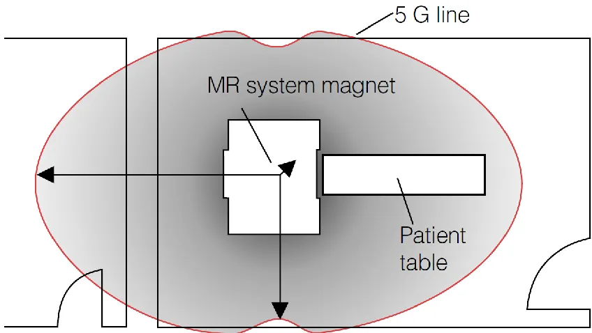
Figure 1.3-9: The electromagnetic environment of an MRI scanner, the MR environment, is defined to be the volume of space enclosed by the 5 Gauss line produced from the MR scanner. The 5G line extends in three dimensions around magnet bore [44]. Reprinted with permission from ECRI Institute, Plymouth Meeting, Pennsylvania.

1.3.5 The Screening Process for Patients Entering the MR

Environment

The American College of Radiology developed the guidance document for safe MR practices. Though not a regulatory standard, the four zones model is widely used in the screening processes for individuals proceeding from the outside the MR facility in zone one to the scanner room in zone four [44-45]. The four zones are defined by the ACR as follows [45]:

Zone II – This area is the interface between Zone I and Zone III. Patients are under supervision by MR personnel and are not free to move throughout Zone II at will. Patient screening and ferromagnetic detection occurs at this zone. Like Zone I, no field higher than 5 G in Zone II.

Zone III – This area is not freely accessible by unscreened non-MR personnel. Ferromagnetic objects or equipment in this area can result in serious injury or death as a result of interactions between individuals or equipment and the MR environment. All access to Zone III, which often provide access to Zone IV, is to be strictly physically restricted, controlled by, and under the supervision of MR personnel. Starting in Zone III, there begin to be fields higher than 5 G.

Zone IV – This is the room that contains the MR scanner and is accessed through Zone II or III. The highest field strengths are within this room and so, there is also the greatest risk. All ferromagnetic objects that have been identified to pose as a risk are excluded from this room.

The MR screening process is a multilevel process consisting of a preliminary interview followed by an MR screening form. The form contains questions to determine the medical history and metal exposure history of the patient. There are two levels of MR personnel. Level 1 personnel have passed minimal safety education and can work within zone 3 and level 2 personnel have received extensive training and education in the broader aspects of MR safety. Those who qualify to be level 2 personnel (i.e. MR technologists, radiologists, and certified MR physicists) are tasked with conducting physical examinations for signs of medical implants if the medical history of the patient cannot be obtained [44,45].

Before entering zone 3, any individual undergoing an MRI scan is required to remove all readily removable metallic personal items and devices on their body. The screening process should have ensured that all non-readily removable metallic items have been considered and have been identified as compatible in the MR environment. Any individual not undergoing an MR scan is subject to the same screening process before entering zone 3 or 4.

1.4 Medical Devices

The standard published by the International Organization for Standardization, ISO 13485 is in regard to medical devices and quality management systems. It is an internationally agreed standard for quality management in the medical device industry [31]. To paraphrase the ISO document, the following is a definition of a medical device [26].

Medical Device – any instrument apparatus, machine, implant, material, or other similar or related article, intended by the manufacturer to be used, alone or in combination, for human beings for one or more of the specific purpose or purposes of diagnosis, prevention, monitoring, treatment, or alleviation of disease or injury, supporting or sustaining life.

ISO 13485 definition is also used by ASTM International in the test standards for magnetically induced displacement force and torque as well as for medical device marking [14,15,26]. The ASTM standard for RF induced heating from passive implants uses a definition for an implant in medicine [13]. It stipulates that an implant is an object, structure, or device intended to reside within the body for diagnostic, prosthetic, or other therapeutic purposes. The Medical Devices Bureau of Health Canada states that a medical device could be any product used in the treatment, mitigation, diagnosis or prevention of a disease or abnormal physical condition [24]. Health Canada uses the ISO 13485 when it comes to quality system certificates.

CDRH proposed the following set of terminology for classifying medical devices by safety in an MR scanner [25].

MR Safe - An item that poses no known hazards in all MR environments. MR Safe items are composed of materials that are electrically conductive, metallic, and non-magnetic [25,26].

MR Conditional - An item that has been demonstrated to pose no known hazards in a specified MR environment with specified conditions of use. To be present within an MR scanner, the field conditions that need to be known include, but are not limited to, the field strength, spatial gradient, dB/dt, RF fields, and SAR [25,26].

MR Unsafe - An item that is known to pose hazards in all MR environments [25]. An item which poses unacceptable risks to the patient, medical staff or persons within the MR environment [26].

1.4.1 Electromagnetic Material Properties

Some material properties that can result in interactions with the EM environment from the MR scanner include conductivity and resistivity, permittivity, and permeability. Electrical conductivity represents a material’s ability to conduct an electric current while conversely, resistivity is how strongly a material resists the flow of an electric current and can be found by taking the reciprocal of the conductivity. An excellent conductor such as copper, the material commonly used in coil windings, has a conductivity of 6 × 107 S/m and resistivity of 1.68 × 10−8 _{Ωm at 20℃. Air on the other hand, a poor conductor, has a}

resistivity on the order of 1016 _{Ωm and a conductivity on the order of 10}−15 _{S/m at 20℃.}

The permittivity of a material describes the amount of charge needed to generate electric flux in that material and is denoted by 𝜀_𝑚. The permittivity of vacuum is constant and denoted by 𝜀0. The relative permittivity is the ratio of 𝜀𝑚 to 𝜀0 and is denoted by 𝜀𝑟.

The permeability of a material is the measure of a material’s ability to allow an external magnetic field to pass through it. It can be described as the degree of magnetization that a material obtains when placed in an external magnetic field. The permeability of a material is denoted by 𝜇_𝑚 while the permeability of vacuum is 𝜇₀. The relative permeability of a material is the ratio of 𝜇_𝑚 to 𝜇₀ and is denoted by 𝜇_𝑟. A related concept is the magnetic susceptibility of a material, 𝜒𝑚, which is a measure of how much a material

will become magnetized when exposed to an external magnetic field. Mathematically, 𝜒_𝑚 is a dimensionless quantity that is the proportionality constant found by the ratio of the net magnetization, 𝐌, and the magnetic field strength, 𝐇 [56].

Diamagnetism – Materials of this kind exhibit no net magnetic dipole moment until they are exposed to an external magnetic field. When an external field is applied, these materials show a magnetic moment that opposes the applied field. Diamagnetic materials repel the external magnetic field and have a negative magnetic susceptibility. Diamagnetism is an effect that occurs in all materials however, the effect is overcome in paramagnetic and ferromagnetic material that possess stronger attraction to the external field. Diamagnetic substances include inert gases, copper, and silver [16].

Paramagnetism – Without an external magnetic field present, the magnetic moments in a paramagnetic material exist in random orientations that cancel each other out and thus have no net magnetic moment. When an external field is applied however, the magnetic moments of paramagnetic substances align in the direction of the field and are denoted by a positive magnetic susceptibility. Paramagnetic materials affect the magnetic field in a positive way and are attracted by the applied field [16].

Ferromagnetism – When ferromagnetic material, come into contact with an external magnetic field, there is strong attraction and alignment. Even when taken out of the field, ferromagnetic materials retain their magnetization, are permanently magnetized and become permanent magnets [16].

Figure 1.4-2: The spectrum of magnetic susceptibility divided into diamagnetic, paramagnetic, and ferromagnetic regions with well-known materials labelled [7]. The ferromagnetic region of the section begins at 𝜒_𝑚 > 10−2_{. Medical implant grade metals}

such as commercially pure titanium and stainless steel are shown in the paramagnetic region [7,27,28]. Although these materials are not ferromagnetic, they are outside of the region of MRI compatibility. Reprinted with permission from John Wiley and Sons, reference 56.

1.4.2 Interactions with an MR Scanner

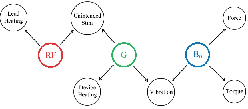
Figure 1.4-3: Possible device interactions with the static magnetic field, B0, pulsed

gradient and radiofrequency fields. This diagram was retrieved from the standard, ISO/TS 10974, which offers methods for evaluating all of the interactions shown as well as device malfunction from output fields individually and in tandem [11]. ASTM International has also published test standards for magnetically induced force and torque, and RF induced heating in passive implants [13-15]. The International Electrotechnical Commission has published test standards on the safety and performance of medical electric equipment in MRI [34]. Copied by Xiao Fan Ding with the permission of the Standards Council of Canada (SCC) on behalf of ISO.

1.4.2.1 Radiofrequency Interactions

Theprimary concern from exposure to the RF fields is heating, which can occur in human tissue as well as in the tissue regions surrounded by passive medical implants and the leads of active implanted medical devices (AIMDs) [11,15,17]. Passive implants do not require a supply of electricity while active implants do.

deposited into the body after an applied RF pulse in MR imaging. The energy deposited manifests as joule heating owing to the small electrical conductivity of biological tissue [57].

The characteristics of tissues in relation to the incident RF wavelength are important factors in determining power deposited into tissue by and RF pulse. If the tissue is large, in surface area, in relation to the incident wavelength, RF energy is predominantly absorbed on the surface. Conversely, if the tissue is small compared to the wavelength, there is little absorption at all [58].

RF induced temperature rise in tissue is related to the SAR, a measure of power deposited into tissue by RF exposure. SAR is not a measure of heating, though it is directly proportional to the rate of change of temperature. SAR is the RF power absorbed per unit mass of an object. The expression for SAR is given in equation 1.4-1 where 𝜎 is the conductivity of the material, 𝐸 is the electric field amplitude, and 𝜌 is the density of tissue [9].

The rate of the change of temperature in tissue as a response to SAR is given by equation 1.4-2 where 𝑇 is the temperature, 𝑡 is time, and 𝐶 is the specific heat capacity and 𝐶_water ≅ 4186 J/(kg ∙ ℃) [9].

The International Electrotechnical Commission (IEC) defines four measures of SAR [9],

Whole-body – SAR averaged over the total mass of the patients’ body over a specified time. The limit is 2 W ∙ kg−1 in normal operation.

Partial-body – SAR averaged over the mass of the patients’ body that is exposed by the

volume RF transmit coil and over a specified time. The limit is 2-10 W ∙ kg−1 in normal operation, depending on the amount of exposed patient mass.

SAR =𝜎𝐸

2

2𝜌 (1.4-1)

d𝑇

d𝑡 =

SAR

Head – SAR averaged over the mass of the patients’ head and over a specific time. The

limit is 3.2 W ∙ kg−1 _{in normal operation.}

Local – SAR averaged over any 10 g of patient body and over a specific time. The limit is 10-20 W ∙ kg−1_{, depending on the part of the body.}

The IEC SAR limits are for an averaging time of 6 min, under normal operating mode, and SAR values over any 10 s period cannot exceed three times the stated values [9]. Normal operating mode is the mode of operation of MR equipment in which none of the outputs have a value that can cause physiological stress to patients [11,34]. Normal operating mode is in the absence of additional sources that can cause stress/harm to patients such as medical implants. With the presence of medical implants, passive or active, RF induced heating in tissue can be enhanced. As opposed to normal operating mode, first level controlled operating mode is the operation of MR equipment under medical supervision appropriate to the patient’s condition. Second level operating mode requires ethics approval from an institutional review board and is typically for human research [34]. It should be noted that a single RF pulse can produce a large enough instantaneous SAR that exceeds SAR limits. A single pulse however, is unlikely to provide sufficient energy to result in significant temperature rise [9].

1.4.2.2 Gradient Interactions

Foreign material interacting with the pulsed gradients during MRI may experience heating, vibrations, and voltages. Biological tissue interacting with the pulsed gradients may experience PNS. Due to the temporally changing gradient magnetic field, dB/dt, eddy currents may form on conductive material. Not only conductive components that make up an implant in a patient, but also the conductive tissue, nerves, of the patient [9,11]. Device interactions may lead to harm, discomfort, or malfunction [11]. PNS causes discomfort and becomes hazardous when occurring near cardiac tissue [17].

Heating occurs due to the induced eddy currents from the temporally changing magnetic field [11]. An alternative name for this effect may be eddy current induced heating [10]. Following Faraday’s law of induction, the change of the magnetic field through the suitable devices induces eddy currents and the material subsequently converts electric energy into thermal energy [17,59]. The effect of heating increase with distance from the magnetic isocentre [10].

Gradient induced vibrations are most common on conductive planar surfaces and are caused by the time varying magnetic moments produced from the aforementioned induced eddy currents. Vibrations are a potential for patient harm as they may cause devices to malfunction. In the absence of conductive surfaces, there is little likelihood of induced vibrations [11]. Apart from vibrations, when the induced magnetic moments interact with the static field, there is the potential for induced torque apart from the induced static torque from device interaction with static field [9].

Gradient induced electric potentials, or gradient induced voltages, can occur within a single AIMD lead, between AIMD leads, or between electrodes and a conductive AIMD enclosure. These voltages, when in contact with adjacent tissue, can cause harm to the patient. As with all the aforementioned device interactions, device malfunction is also a possibility [11,33].

limit is on a 20-cm-radius cylinder surrounding the patient where 𝑡_rectangle is the duration of a rectangular dB/dt pulse [9].

1.4.2.3 Magnetically Induced Displacement Force

The static field gradient, the difference in static field strength around the scanner, can induce a displacement force on an object [9,13]. Ferromagnetic objects can experience an induced force strong enough such that they become airborne as projectiles [16]. Assume that a device has an overall magnetic dipole moment of 𝐦 is placed in a spatially varying magnetic flux density, 𝐁, the magnetic force, 𝐅_𝐦, induced can be described by equation 1.4-4 [9].

When the magnetic field is varying only in the z-direction and that 𝑚_𝑧 is the only component of the magnetic moment, the magnetic force expression becomes equation 1.4-6.

Further considering that a device of volume, 𝑉, and saturation magnetization of, 𝑀_𝑠, the magnitude of magnetic force becomes equation 1.4-7.

d𝐵

d𝑡|_max = (16

T

s) (1 +

0.36 × 10−3 s

𝑡_rectangle ) (1.4-3)

𝐅_𝐦= (𝐦 ∙ ∇)𝐁 (1.4-4)

𝐅_𝐦= ( (𝑚𝑥 𝜕𝐵_𝑥 𝜕𝑥 + 𝑚𝑦 𝜕𝐵_𝑥 𝜕𝑦 + 𝑚𝑧 𝜕𝐵_𝑥 𝜕𝑧) 𝐱̂ (𝑚_𝑥𝜕𝐵𝑦 𝜕𝑥 + 𝑚𝑦 𝜕𝐵_𝑦 𝜕𝑦 + 𝑚𝑧 𝜕𝐵_𝑦 𝜕𝑧 ) 𝐲̂ (𝑚_𝑥𝜕𝐵𝑧 𝜕𝑥 + 𝑚𝑦 𝜕𝐵_𝑧 𝜕𝑦 + 𝑚𝑧 𝜕𝐵_𝑧 𝜕𝑧) 𝐳̂) (1.4-5) 𝐅𝐦 = 𝑚𝑧 𝜕𝐵_𝑧

𝜕𝑧 𝐳̂ (1.4-6)

𝐹𝑚 =

𝑀_𝑠𝑉 𝜇0

𝜕𝐵_𝑧

In equation 1.4-7, 𝜇₀ is the permeability of vacuum. This force is proportional to the static field of the MR scanner [16].

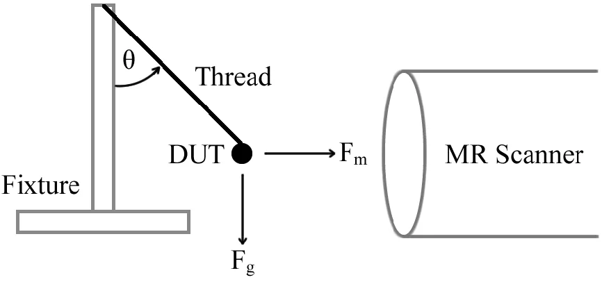
The standard test for magnetically induced displacement force is performed by measuring the deflection angle of a device under testing (DUT). The DUT is attached by a thread of negligible mass to a fixture. The primary measurement tool is a protractor. All material used, other than the DUT, should not interact with the MR environment [9,13]. Figure 1.4-4 shows the schematic of a deflection test for magnetically induced displacement force. If the deflection angle, 𝜃, is less than 45 deg, then the induced force from the scanner poses no more risk than the force experienced everyday from the Earth’s gravity. It should be noted that 45 deg is not an acceptance criterion but rather, a conservative reference point [13]. For each DUT, an acceptance criterion unique to that device needs to be determined.

Figure 1.4-4: The basic schematic of the deflection test method used measure magnetically induced displacement force [9]. The DUT, the black circle, experiences a magnetically induced force, 𝐅_𝐦, as well as its own weight, 𝐅_𝐠. 𝜃 is the deflection angle.

The force ratio is shown in equation 1.4-9 where 𝐹_𝑚 was retrieved from equation 1.4-7 and the weight of an object can be calculated from 1.4-8.

1.4.2.4 Magnetically Induced Torque

Apart from a magnetically induced force, the other major interaction between material and the static field is a magnetically induced torque. The possibility of torque induced on foreign material entering the static field environment of the scanner is the only concern of this thesis.

Like the displacement force, torque induced on a device is due to interactions with the static field of the MR scanner. A magnetic torque is induced on non-spherical magnetic objects that have magnetizations not precisely distributed along the axis of the magnetic field [9]. A sphere of linear magnetic material will have an induced torque of zero and is shown in appendix A.4.

The torque on non-spherical objects will be in the direction such that the longest dimensions of the object will try to align with the static field [9]. For example, a cylinder placed in a uniform magnetic field, 𝐇_𝟎, will experience an induced torque. The cylinder is considered an idealized device given its simple geometry. The field is assumed to be along the direction of the MR bore, the z-direction, and the cylinder is assumed to be uniformly magnetized with a saturation magnetization, 𝑀𝑠, in the xz-plane. The device has rotated 𝜃

degrees away from the x-axis and 𝑀𝑠 is 𝛼 degrees away from the normal. The relevant

magnetic energies are those due to external and normal, 𝑁_𝑛, and transverse, 𝑁_𝑡, demagnetizing fields. The total magnet static energy per volume, 𝑊_𝑇, is therefore given by equation 1.4-10.

𝐹_𝑔 = 𝜌𝑔𝑉 (1.4-8)

Force Ratio =𝐹𝑚

𝐹_𝑔 =

𝑀𝑠 𝜇₀𝜌𝑔

𝜕𝐵𝑧

At equilibrium, it is required that the angular of change of 𝑊_𝑇 with respect to 𝛼 is zero. Equation 1.4-10 then becomes,

By making the definition 1.4-12, equation 1.4-11, the energy minimization, can be rewritten as 1.4-13.

The torque about the y-axis is given by 1.4-14.

The maximal amplitude of the torque is 1.4-15.

In equations 1.4-14 and 1.4-15, 𝑉 is the volume of the device.

One method of measuring the static field induced torque is to place a device on a platform suspended by torsional springs [9,14]. This method was outlined in a previous version of the ASTM standard for measuring torque which, as of 2017, has been updated to include alternative methods. The torque measured using torsional springs is proportional to the deflection angle of spring from the equilibrium position. The angular dependence of the torque is determined by measurement of the deflection angle as a function of the device position [9]. The acceptance criterion for the torsional spring torque tests is determined by the product of the longest dimension of the device and its weight. Should the magnetically induced torque be less than this criterion, then the induced torque poses no greater threat

𝑊_𝑇 = −𝑀𝑠

2

2𝜇₀(𝑁𝑛− 𝑁𝑡) sin

2_{𝛼 − 𝑀}

𝑠𝐻0sin(𝜃 + 𝛼) (1.4-10)

𝑊𝑇 = −

𝑀_𝑠2 2𝜇0

(𝑁𝑛− 𝑁𝑡) sin(2𝛼) − 𝑀𝑠𝐻0cos(𝜃 + 𝛼) = 0 (1.4-11)

𝛽 = 𝑀𝑠

2𝜇₀𝐻₀(𝑁𝑛− 𝑁𝑡) (1.4-12)

𝛽 sin(2𝛼) + cos(𝜃 + 𝛼) = 0 (1.4-13)

𝜏_𝑦 = 𝑀_𝑠𝐻₀cos(𝜃 + 𝛼) × 𝑉 (1.4-14)

𝜏_𝑚𝑎𝑥 = 𝑀𝑠

2

than the torque induced everyday from the Earth’s gravity. Similar to induced force, this criterion is a conservative reference point [9,14].

Apart from the focus of this thesis, the induced eddy currents on conductive material is another source of torque [9]. This effect can be observed by measuring the time required for a sheet made out of a good conductor to fall flat in the static field. Eddy current torque is not believed to pose a safety issue in MRI but has been reported for certain devices such as metallic heart valves [59]. Eddy current torque was not considered in the studies presented in this thesis.

1.5 Electromagnetic Interactions Relevant to Torque

Electromagnetism is the branch of physics that studies the relationship between electricity and magnetism (EM). The fundamental concepts of EM used throughout this thesis are discussed in this subchapter. Section 1.5 relies heavily on Electricity & Magnetism by Munir H. Nayfeh and Morton K. Brussel and Introduction to Electrodynamics by David J. Griffiths [22,23].

Relationships Between Electromagnetic Quantities

The terms magnetic field is often used to describe different but closely related quantities, 𝐁 and 𝐇. The magnetic field, 𝐁, is also called the magnetic flux density and is given in units of tesla, T. The magnetic field, 𝐇, is also called the magnetic field strength is given in units of amperes per meter, A

m. The relationship between 𝐁 and 𝐇 is given by

equation 1.5-1.

In the above equation, 𝜇0 is the magnetic permeability in a vacuum and is constant at

4𝜋 × 10−7 H

m. 𝐌 is the magnetization in units of A

m. By definition, the magnetization is the

density of magnetic dipole moments in magnetic material, shown in equation 1.5-2.

This thesis primarily examines materials in the paramagnetic range. Materials of this variety have a magnetization, 𝐌, sustained by the field that it is in. When the external field, 𝐇, is removed, 𝐌 disappears as well. The magnetization, being proportional to the field, can be expressed in terms of 𝐇 using the magnetic susceptibility, 𝜒, as a proportionality constant.

Materials that obey equation 1.5-3 are known as linear magnetic material. Substituting equation 1.5-3 into equation 1.5-1 it can be shown that in linear material, 𝐁 is proportional to 𝐇 by the magnetic permeability of the material.

The ratio of 𝜇_𝑚 to 𝜇₀ is the relative permeability, 𝜇_𝑟. The relative permeability itself is can be written in terms of the relative susceptibility.

1.5.1 A Sphere of Linear Magnetic Material

A classic EM problem involves finding the magnetic flux density, 𝐁, inside and outside of a sphere of linear magnetic material embedded a uniform external magnetic field, 𝐇_𝟎. The sphere has a magnetic permeability of 𝜇₁ and the medium that it has been placed in has a magnetic permeability of 𝜇₂. The sphere is placed at the origin with 𝐇_𝟎pointing along the z direction. Appendix A.2 details the solution for 𝐁 inside and outside of the sphere.

𝐌 =∑ 𝐦

𝑉 (1.5-2)

𝐌 = 𝜒𝐇 (1.5-3)

𝐁 = 𝜇_𝑚𝐇 (1.5-4)

𝜇_𝑟 =𝜇𝑚

𝜇0

= 1 + 𝜒 (1.5-5)

𝐁_𝐢𝐧 = 3𝜇𝑟

Equations 1.5-6 and 1.5-7 are true for when 𝐇𝟎is along the z direction. For a more general

solution when 𝐇_𝟎 and also 𝐁_𝟎is inan arbitrary direction, 𝐁_𝟎= 〈𝐵0𝑥𝐱̂ 𝐵0𝑦𝐲̂ 𝐵0𝑧𝐳̂〉

the magnetic flux density inside and outside of the sphere would be given by the following,

In equation 1.5-8, the magnetic flux density inside of the sphere is equal in magnitude to equation 1.5-6. Though the direction of 𝐁 inside the sphere changes as 𝐁_𝟎changes, the magnitude remains the same regardless of direction.

𝐁𝐨𝐮𝐭 =

(

𝐵₀𝑅3𝜇𝑟− 1 𝜇𝑟+ 2

3𝑥𝑧 (𝑥2_{+ 𝑦}2 _{+ 𝑧}2₎5₂

𝐱̂

𝐵₀𝑅3𝜇𝑟− 1 𝜇_𝑟+ 2

3𝑦𝑧 (𝑥2_{+ 𝑦}2_{+ 𝑧}2₎5₂

𝐲̂

𝐵₀(1 + 𝑅3𝜇𝑟− 1 𝜇_𝑟+ 2

𝑥2 _{+ 𝑦}2_{− 2𝑧}2 (𝑥2_{+ 𝑦}2_{+ 𝑧}2₎5₂

) 𝐳̂ )

(1.5-7)

𝐁_𝐢𝐧 = 3𝜇𝑟

𝜇_𝑟+ 2(

𝐵_0𝑥𝐱̂ 𝐵_0𝑦𝐲̂ 𝐵_0𝑧𝐳̂

) (1.5-8)

𝐁𝐨𝐮𝐭

=

(

(𝐵0𝑥+ 𝑅3

𝜇_𝑟− 1

𝜇_𝑟+ 2(

3𝑥(𝑦𝐵0𝑦 + 𝑧𝐵0𝑧) − 𝐵0𝑥(𝑦2+ 𝑧2 − 2𝑥2) (𝑥2_{+ 𝑦}2_{+ 𝑧}2₎5₂

)) 𝐱̂

(𝐵0𝑦+ 𝑅3

𝜇_𝑟− 1 𝜇𝑟+ 2

(3𝑦(𝑥𝐵0𝑥+ 𝑧𝐵0𝑧) − 𝐵0𝑦(𝑥

2 _{+ 𝑧}2_{− 2𝑦}2₎ (𝑥2_{+ 𝑦}2_{+ 𝑧}2₎5₂

)) 𝐲̂

(𝐵_0𝑧+ 𝑅3𝜇𝑟− 1 𝜇𝑟+ 2

(3𝑧(𝑥𝐵0𝑥+ 𝑦𝐵0𝑦) − 𝐵0𝑧(𝑥

2_{+ 𝑦}2_{− 2𝑧}2₎ (𝑥2_{+ 𝑦}2_{+ 𝑧}2₎5₂

)) 𝐳̂ )

1.5.2 An Infinitely Long Cylinder of Linear Magnetic Material

Another classic EM problem is finding 𝐁 inside and outside of an infinitely long cylinder of linear magnetic material embedded in an arbitrary 𝐇𝟎. The magnetic

permeability of the cylinder and surrounding are 𝜇₁ and 𝜇₂. Appendix A.3 details the solution for 𝐁 inside and outside of the cylinder when the direction of 𝐇_𝟎is perpendicular to the longitudinal axis.

The solution for 𝐁 when 𝐇𝟎is parallel to the cylinder is the following,

Equations 1.5-10 and 1.5-11 are true for when 𝐇_𝟎is perpendicular to the cylinder and equations 1.5-12 and 1.5-13 are true when 𝐇_𝟎is parallel. As was with the case of a sphere, when 𝐇𝟎 and also 𝐁𝟎 is in an arbitrary direction, the magnetic flux density inside and

outside of the cylinder would be given by the following,

𝐁_𝐢𝐧= 2𝜇𝑟

𝜇_𝑟+ 1𝐵0𝐱̂ (1.5-10)

𝐁𝐨𝐮𝐭 =

(

𝐵₀(1 + 𝑅2𝜇𝑟− 1 𝜇_𝑟+ 1

𝑥2 _{− 𝑦}2 (𝑥2_{+ 𝑦}2₎2) 𝐱̂ 𝐵₀𝑅2𝜇𝑟− 1

𝜇𝑟+ 1

2𝑥𝑦 (𝑥2_{+ 𝑦}2₎2𝐲̂

0 )

(1.5-11)

𝐁_𝐢𝐧= 𝜇_𝑟𝐵_0𝑧𝐳̂ (1.5-12)

𝐁_𝐨𝐮𝐭 = 𝐵_0𝑧𝐳̂ (1.5-13)

𝐁𝐢𝐧 =

( 2𝜇_𝑟 𝜇𝑟+ 1

𝐵0𝑥𝐱̂ 2𝜇_𝑟

𝜇_𝑟+ 1𝐵0𝑦𝐲̂ 𝜇_𝑟𝐵_0𝑧𝐳̂ )

(1.5-14)

𝐁𝐨𝐮𝐭 =

(

(𝐵_0𝑥+ 𝑅2𝜇𝑟− 1 𝜇_𝑟+ 1(

2𝑥𝑦𝐵0𝑦 + 𝐵0𝑥(𝑥2− 𝑦2)

(𝑥2_{+ 𝑦}2₎2 )) 𝐱̂

(𝐵_0𝑦+ 𝑅2𝜇𝑟− 1 𝜇_𝑟+ 1(

2𝑥𝑦𝐵0𝑥+ 𝐵0𝑦(𝑦2− 𝑥2)

(𝑥2_{+ 𝑦}2₎2 )) 𝐲̂

𝐵_0𝑧𝐳̂ )