A Method for Mapping Vegetation Utilizing
Multivariate Statistical Techniques
TERRY MCLENDON AND BILL E. DAHL
Abstract
Principal component analysis and stepwise discriminant analy- sis were used to map the vegetation of the Pat Welder Ranch on the Texas Coastal Plains into 5 vegetation types based on relative frequency data of the major plant species. These 5 types were shown to be subdivisions of 2 plant communities previously reported for the area by researchers utilizing conventional map- ping techniques. In addition to separating the 5 types and classify- ing the 140 sample points into their respective types, the technique provided a key for field separation of the types based on 3 vegeta- tive variables, and provided indicator species values for rapid field identification of the types. The technique is presented as a means of mapping vegetation with a minimum of human bias, a maximum of repeatability and information content, and maximum applicability.
The traditional method of mapping the vegetation of an area has been for a worker to separate various locales into vegetation types, communities, or associations based on observed similarities or dissimilarities in species distributions or structure. This has the disadvantage of being based on personal subjective biases. An improvement over this “eyeballing” method can be made by the addition of quantitative data on which decisions are made; fre- quency, biomass, cover, trunk or stem diameter, etc. However, much of the qualitative judgement remains in deciding how the data are to be used, what constitutes sufficient differences to separate groups, and what weight should be given the various measurements. Given the same data, but working separately, it is quite possible for 2 workers to arrive at different conclusions concerning the same area.
It would seem desirable, therefore, to develop a method of mapping vegetation, or any resource, which would minimize the personal bias of the investigator, maximize the repeatability of the results, maximize the information content, and be applicable to a maximum number of situations. Oneapproach to such a method is presented.
Description of Area
This study was conducted on the Pat Welder Ranch in San Patricia County on the Texas Coastal Plains. The area is relatively level except where intersected by creeks and rivers. The ranch is drained by intermittent streams which flow into the Aransas River 3 km to the northeast. Elevation ranges from 4 to 20 m above sea level.
Thornthwaite (1948) classified the climate of the area as dry subhumid and megathermal. Total annual precipitation for the study area averages 835 mm with a high of 1,486 mm and a low of 346 mm. The mean January minimum temperature is 8O C and the mean July high temperature is 33OC (United States Weather Bureau 1961).
Authors are range and ecological consultant, I20 I S. Circle Drive, Kingsville, Tex. 7836% and professor, Department of Range and Wildlife Management, Texas Tech University, Lubbock.
This paper is publication number T-9-277 of the College of Agricultuml Sciences, Texas Tech University. The cooperation and support provided by P.H. Welder, Victoria, is gratefully acknowledged.
Manuscript received December 14, 1981.
Godfrey et al. (1973) described the soils of the study area as poorly to moderately drained, cracking clayey soils and mostly poorly drained soils with loamy surface layers and cracking clayey subsoils. Tharp (1926, 1939) placed the study area into a Coastal Prairie vegetation type, described as large stretches of level grass- land, with local areas of well-developed woodland. Box( 196l)and Box and Chamrad (1966) described the plant communities on the adjacent Welder Wildlife Refuge. The 16 communities that they separated were:
Communities of clay and clay loam sites
Mesquite-buffalograss, Chaparral-bristlegrass, Prickly pear- shottgtass, Halophyte-cactus, Paspalum aquatic weed, Cordgrass, and Huisache-buffalograss
Communities of sandy and sandy loam sites
Bunchgrassannual forb, Colubrina-bunchgrass, Huisache- bunchgrass, Chittimwood-hackberry, and Live oak- chaparral
Communities of bottomland sites
Hackbetry-anacua and Woodland-spiny aster complex Communities of aquatic sites
Spiny aster-Longtom and lakes and ponds.
The Welder Wildlife Refuge borders on the Atansas Rivet and as a result has a greater complexity of plant communities than might normally be expected for an area of its size. The river bottom and associated aquatic sites account for 8 of the 16communities and do not occur in significant amounts on the Pat Welder Ranch.
Methods
During the summers of 1970 and 1973, 140 points were selected on aerial photographs of the Pat Welder Ranch by a stratified random process, with stratification based on pastures. A sample point was designated on the ground corresponding to each of the points on the photographs. Ten 40 X 40 cm plots were located along a north-south transect from each point at 5-m intervals. and presence of all species within the plots were recorded. A grass or forb species was recorded as present if it was tooted within the frame and a brush species was recorded as present it if was either tooted in ot its canopy covered any part of the area within the plot frame. From the raw frequency data, a relative frequency value was computed for each species at each point by dividing the total number of plots, at that point, in which the species occurred by IO. The variable ‘number of species’ was computed by determining the total number of individual species which were found to occur in the IO-plot total at each point.
It is recognized that frequency data are not always desirable as the single criterion for vegetation mapping. The use of such in this study was the result of previous data collection in a limited time span for completion of the work. However, the mapping technique remains the same whether frequency, density, covet, biomass, or any other variable ot combination of variables is used.
was Texas broomweed (Xanthocephalum texanum), which was retained because it was so widely distributed and occurred with such high frequencies that the yearly variation was considered to be small. A total of 35 variables were then available for use in the statistical analysis: number of species, the relative frequencies for the 33 major perennial species, and the frequency of Texas broomweed.
All statistical analyses used in the mapping technique assume either a normal or a multivariate normal distribution for the variables. The univariate distributions for each of the variables were estimated by plotting the frequency classes of the values of the sum of the 140 observations. Of the 35 potential variables, only 9 had any possibility of a normal distribution. The normality of these 9 distributions were tested by the Chi-Square Goodness of Fit Method (Snedecor and Cochran 1967). Of these 9 variables, 6 were rejected at the 95% probability level. The three remaining were number of species, mesquite (Prosopisglandufosa) frequency, and ragweed (Ambrosiapsilostachya) frequency. The knotroot bristle- grass (Setariageniculata) frequency variable was a marginal rejec- tion. A shift of only one value out of the 140 (an 8 to a 7 or less) would have been sufficient to keep from rejecting the null hypothe- sis. Consequently, the bristlegrass frequency variable was not elim- inated from the model; the advantage of increasing the variables to 4 was considered to outweigh the disadvantage of the slight devia- tion from a normal distribution. It should be recognized that the fact that the distributions of the 4 variables can be estimated to be normal (or nearly so) does not indicate that their combined distri- bution is multivariate normal. It does, however, increase the probability.
Once the model was reduced to contain only variables approxi- mately normally distributed, 2 procedures remained: (I) to separ- ate the I40 locations (samples) into p significantly different groups, and (2) to describe these p groups and test the classification of the
140 locations. Principal component analysis (BMD-OIM, Dixon 1973) was used for the original classification of the 140 locations into groups. Principal component analysis is a multivariate tech- nique that was used in this procedure to accomplish two goals: reduce the sample variables (some of which are often significantly correlated) into a smaller set of independent linear combinations (the principal components) in such a manner as to maximize the variance between these combinations, and secondly to initially separate the observations into groups. This first goal results in information content being maximized and correlation minimized. The second goal is required as a result of the fact thatdiscriminant analysis requires an initial grouping of the observations. Basing this initial grouping on principal component analysis reduces a major source of human bias. Overall and Klett (1972) suggested that principal component analysis be used where the aim is to describe differences between observations in a heterogeneous sam- ple in terms of a relatively few composite variables. Seal (1964) listed a number of limitations to the use of principal components and these should be considered before the method is applied, with alternative methods utilized if required. Perhaps the most impor- tant of these limitations is that if the off-diagonal elements of the correlation matrix are approximately equal, then the interpretive value of a principal component analysis of this matrix is questiona- ble (Seal 1964).
The 140 locations were plotted on a 2-dimensional graph on the basis of their respective values of the first 2 principal components, with the first principal component plotted along the Xaxisand the second along the Y axis. These two components accounted for 61 yc of the total variance.
The maximum number of groups which can be separated by discriminant analysis is one more than the number of variables used. Since there were only 4 vegetation variables remaining in the model, the graph of the results of the principal component analysis was divided into 5 equal areas, each area corresponding to one group. The 5 groups were: (I) those points nearest zero for both principal components, (2) those points with a high positive value for component Ye and a high negative value for component Yl, (3)
those points with a high positive value for both components, (4) those points with a high positive value for component Y1 and a high negative value for component Yz, and (5) those points with a high negative value for both components. This method can be com- pared with the 9 group separation used by Overall and Klett (I 972). It should be repeated that the maximum number of initial groups is bounded by the number of variables used in the analysis and the division of the graph is in turn dependent on this number.
Once the graph was divided into the 5 segments, each of the 140 locations was assigned to one of the 5 groups on the basis of its location on the graph. These 5 groups were then entered into a stepwise discriminant analysis(BMD-07M, Dixon 1973). Discrim- inant analysis was used to achieve 3 goals: (I) test for significant differences between the initial groups, (2) final classification of the observations into their respective groups, and (3) description of the groups based on the original sample variables. The group descrip- tions provided measurements of relative similarities between groups, means and variances of the variables within each group, and those variables and their values most useful in group separa- tion and classification of new observations (i.e., indicator species). The significance of the differences between the groups was based on the matrix of F-statistics testing the equality of means between each pair of groups and the classification of individuals was based on the square of the Mahalanobis distance from each group. The discriminant analysis was considered complete when all groups were significantly different from each other (95% level) and all locations were in the propergroups based on minimum Mahalano- bis D2.
Upon the final iteration of the discriminant analysis, each group was considered to be a vegetation type, characterized by those
Fig. 1. Two-dimensionalpresentation of the D-‘-values between the means of thefive vegetation rypes of the Pat Welder Ranch.
species (regardless of distribution) which had the highest frequency values for that group. Each location classified into that type was located on a map of the Pat Welder Ranch. The boundary lines between the types were drawn on the basis of observable differen- ces on aerial photographs between the plotted locations (Fig. 1).
Results and Discussion
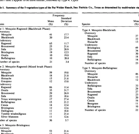
The general aspect of the vegetation of the study area is a Mesquite-mixed brush community. Any subdivision of this gen- eral classification is based on species variation in the mixed brush and understory components. This was accomplished by the dis- criminant analysis. Five significantly different (95% probability level) vegetation types were separated and characterized on the basis of the variables entered. The 5 types and the values of the species with largest frequency values are summarized in Table 1.
Two possible methods for determining the similarities between the types are F-values and Mahalanobis D* values, both taken from the discriminant analysis and presented in Table 2. From these values and the two-dimensional presentation in Figure 1, Types 1 and 2 appear to be most similar, followed by Type 4. Types
3 and 5 are most dissimilar. Types I, 2, 3. and 4 are apparently subdivisions of the chaparral-bristlegrass community reported by Box and Chamrad (1966). Overstory vegetation is composed prim- arily of mesquite and blackbrush (Acacia rigidulu), with various additional overstory species. Understory composition is variable depending on which of the 4 types is studied. Type 5 appears to be similar to the huisache-buffalograss community of Box and Cham- rad (1966) with mesquite density greatly increased.
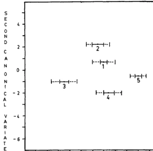
The first canonical variable of the discriminant analysis had an eigenvalue of 4.85 and accounted for 68% of the total dispersion of the observations. This variable was primarily composed of a com- bination of the ragweed and bristlegrass frequency variables. The second canonical variable consisted of bristlegrass-ragweed con- trast and had an eigenvalue of I .90, and when combined with the first canonical variable, accounted for 95% of the total dispersion. Figure 2 presents the means of the 5 types as plotted against the first 2 canonical variables. The confidence intervals shown are based only on the variance of the first variable. From thisdata, it is apparent that Type 3 and Type 5 are separated from the remaining 3 types on the basis of high bristlegrass and ragweed frequencies
Table 1. Summary of the 5 vegetation types of the Pat Welder Ran&San Patricia Co., Texas as determined by multivariate statistical methods.
Species
Frequency Standard Mean Deviation
(%) (%)
Type I. Mesquite-Ragweed (Blackbrush Phase): Overstory
Mesquite 41
Blackbrush 20
Understory
Ragweed 65
Broomweed 25
Sida 23
Bristlegrass I9
Oxalis IO
Buffalograss IO
Number of species 21
Type 2. Mesquite-Ragweed (Mixed brush Phase): Overstory
Mesquite 59
Blackbrush I8
Huisache IS
Granjeno I2
Understory
Ragweed 86
Oxalis 35
Broomweed 29
Sida 22
Texas wintergrass I7
Buffalograss I5
Cassia I4
Bristlegrass I2
Dallisgrass II
Tumble windmillgrass II
Silver bluestem II
Number of species 30
Type 3. Mesquite-Bristlegrass: Overstory
Mesquite 53
Blackbrush I?
Understory
Bristlegrass 61
Ragweed 79
Broomweed 33
Sida I3
Silver bluestem IO
Texas wintergrass IO
Number of species 21
17.7 23.4
11.7 21.6 28.9 12.5 19.0 20.8 3.8
19.8 21.8 21.8 15.8
Il.4 31.7 26.9 18.6 27.4 21.2 12.4 12.6 18.8 21.4 12.6 5.7
21.6 23.4
15.0 15.3 26.8 18.3 15.9 20.0 4.4
Frequency Standard Mean Deviation
Species (%) (o/c)
Type 4. Mesquite-Blackbrush: Overstory
Mesquite Blackbrush Huisache Understory
Bristlegrass Broomweed Ragweed Sida Buffalograss Number of species
Type 5. Mesquite-Buffalograss: Overstory
Mesquite Huisache Blackbrush Understory
Buffalograss Sida Broomweed Ragweed Oxalis Cassia Bentgrass Bristlegrass Number of species
37 27.2
33 29. I
I3 13.7
49 14.1
34 25.5
30 15.6
18 14.6
I4 31.5
23 6.1
46 22.0
I3 12.4
I2 19.4
33 37.6
29 28.0
27 26. I
23 14.6
20 28.1
16 20. I
II 17.8
10 9.8
Table 2. F-values (lower offdiagonal elements) and Mahalmobis D*- values (upper offdiagonal elements) indicating the similarities of the group means of the five vegetation types of the Pat Welder Ranch as pro- vided by discriminant analysis.
Types 1 2 3 4 5
1 - 9.09 18.18 14.52 16.49 2 18.32 - 24.84 27.29 26.76 3 62.51 56.33 - 22.10 48.07 4 35.12 51.54 48.85 - 15.33 5 57.26 63.20 158.57 31.15 -
(Type 3) or low bristlegrass and ragweed frequencies (Type 5). The second canonical variable then separates the remaining 3 types on the basis of a bristlegrass-ragweed contrast. Type 2 has a high ragweed frequency but a low bristlegrass frequency, Type 5 a high bristlegrass and low ragweed frequency, and Type 1 is intermediate in ragweed but low in bristlegrass.
The third canonical variable corresponded to a ragweed vs. (mesquite -I- species number -I- bristlegrass) contrast, had an eigen- value of 0.34, and accounted for 99% of the dispersion when combined with the first 2 variables. The fourth canonical variable was primarily the mesquite frequency variable and had an eigen- value of 0.04. The equations of the 4 canonical variables were:
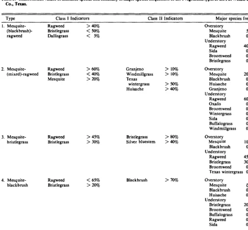
Table 3. Characteristic values of indicator species and summary of major species frequencies of the 5 vegetation types of the Pat Welder Ranch, San Patricia Co., Texas.
Type Class I Indicators Class II Indicators Major species frequencies (%)
2. Mesquite- (mixed)-ragweed
Ragweed > 60%
Bristlegrass <40%
Mesquite > 2%
3. Mesquite- Ragweed > 45% Bristlegrass > 80%
bristlegrass Bristlegrass > 3% Silver bluestem >40%
Granjeno Windmillgrass Texas
wintergrass Huisache
> 10% > 10%
> 50% >40%
I. Mesquite- Ragweed >40%
(blackbrush)- Bristlegrass < 5%
ragweed Dallisgrass < 5%
Overstory Mesquite Blackbrush Understory
Ragweed Sida Broomweed Bristlegrass
Overstory Mesquite Blackbrush Huisache Granjeno Understory Ragweed Oxalis Broomweed Wintergrass Sida Buffalograss Windmillgrass
Overstory Mesquite
Blackbrush Understory
Ragweed Bristlegrass Broomweed
5- 80 o- 70
40-100 0- 80 o- 70 o- 45
20-100 0- 65 0- 60 o- 45
60-100 O-100 0- 85 o- 75 0- 60 0- 60 0- 55
IO- 95 0- 65
45-100 30- 95 o- 90
4. Mesquite- Ragweed < 65%
blackbrush Bristlegrass > 20%
5. Mesquite- Ragweed c 55%
buffalograss Bristlegrass < 30%
Blackbrush > 70%
Bentgrass > 10% Buffalograss > 80%
Cassia >40%
Texas wintergrass 0- 50
Overstory Mesquite Blackbrush Huisache Understory
Bristlegrass Broomweed Buffalograss Ragweed Sida
Overstory Mesquite Blackbrush Huisache Understory
Buffalograss Sida Broomweed
Oxalis Cassia
Raeweed
b- 95 o- 95 o- 40
20- 80 o- 85 o- 75 0- 60 o- 45
5- 90 o- 50 o- 40
O-100 0- 85 0- 80
o- 75 o- 55
o- 50
s
E c .c- 0 N D
2- C A N
o- 0
t--‘--l
‘---‘r’---’
N I C -2- A
L
t---‘---’ t--,--i
t-lpiV -4 - A R I A -6- T
E L , , , , , , , , , , , ,
-6 -4 -2 0 2 L
1
FIRST C ANON ICAL VARIATE
Fig. 2. l%e means and 9.5% confidence intervals of the means (solid lines) and of the observations (broken lines) of the five vegetation types of the Pat Welder Ranch, San Patricia Co.. Texas, based on rhe firsi IWO canonical variables.
CVt = 3.90 - 0.63 (ragweed) - 0.58 (bristlegrass) -I 0.06 (number of species) + 0.03 (mesquite)
CVe = -I .75 -0.54 (bristlegrass) -I- 0.42 (ragweed) -I 0.04 (number of species) - 0.03 mesquite)
CVs = 4.86 - 0.20 ) mesquite - 0.18 (number of species) - 0.16 (bristle- grass) + 0.12 (ragweed)
CVs = -0.09 + 0.44 (mesquite) - 0.07 (number of species) - 0.05 (rag- weed) - 0.04 (bristlegrass)
The low eigenvalues for the third and fourth canonical variables with the corresponding ability of the 2-variable model to account for 95% of the dispersion suggests that the species number and mesquite frequency variables could be eliminated from the model. The approximate F-value however, indicates significance at the 95% level for even the fourth variable, mesquite frequency.
The preceding analysis allows for the following key for the classification of an observation into 1 of the 5 vegetation types based on the 4 variables.
A. Western ragweed frequency less than 50% B. Knotroot bristlegrass frequency less than 25%
Type 5. Mesquite-buffalograss
B. Knotroot bristlegrass frequency greater than or equal to 25% Type 4. Mesquite-blackbrush
A. Western ragweed frequency greater than or equal to 5% C. Knotroot bristlegrass frequency greater than or equal to 40%
Type 3. Mesquite-bristlegrass
C. Knotroot bristlegrass frequency less than 40% D. Number of species less than 25
Type I. Mesquite-(blackbrush)-ragweed D. Number of species greater than or equal to 25
Type 2. Mesquite-(mixed)-ragweed
Table 4 presents a general summary of the frequency values expected to occur for the major species of each of the 5 types, based on the confidence intervals of the means. In addition, 2 classes of indicator species values are presented for the types. The Class 1 values hold true for every location classified into the respective type, i.e., no location can be a given type without meeting these values for that type. The converse, however, is not necessarily true, i.e., a location of a specific type may also meet the Class 1 criteria of another type. Class 11 values hold true only for the specific type listed, e.g., no Type 2 location fits the Class 11 criteria of any other type. Again, the converse is not necessarily true. A location of a given type may exist without meeting the Class 11 indicator values for that type. The usefulness of the indicator values is in rapid identification of an area into its respective vegetation type. If an investigator believes he is in an area of a given type, it must at least fit the Class 1 values. If it also fits the Class II values, it can be validated as that type.
As indicated by the data in Table 3 and Figure 1, Types I and 2 are most similar. Both have overstories dominated by mesquite, with blackbrush the only other major overstory species, and an understory composed primarily of forbs, with bristlegrass fre- quency being relatively low. Type 2 appears to be the more deve- loped of the two. The overstory is more complex and more dense. Mesquite frequency increases and huisache (Acacia farnesiana) and granjeno (Celris pallida) become major components. Black- brush and huisache were shown by the discriminant analysis to be significantly negatively correlated. Grasses also increase in impor- tance in Type 2, with 3 species becoming major components. The increase in huisache frequency and the frequencies of the 3 grass species suggest improved soil moisture conditions for Type 2 as compared to Type I. Livestock grazing might also have contrib- uted to the differences, with Type I being a more severely grazed phase of Type 2.
Types 4 and 5 are the next most similar types, with similar differences as were shown for Types 1 and 2. The overstory of Type 4 is composed of similar amounts of mesquite and blackbrush, with some huisache. In Type 5, blackbrush frequency decreases to the level of huisache. This may also indicate improved moisture condi- tions for Type 5. Observations over large areas of South Texas and northeastern Mexico indicate that as sites become drier, often because of a decrease in soil depth, blackbrush increases in density. Bristlegrass is the most frequent understory species in Type 4, and buffalograss (Buchloe dactyloides) is of much lower density. The opposite is true for Type 5, buffalograss is the most frequent grass species and bristlegrass is a minor component. The frequency ranking of the forb species is also reversed for the two types.
Type 3 is the most distinct of any of the 5 types. It has mesquite and blackbrush as major overstory species and ragweed and bris- tlegrass as major understory species, as does Type 4. This may indicate that Type 3 is a development of Type 4, further developing those differences which separated Type 4 and Type 5. The ragweed- bristlegrass understory structure is most developed within Type 3.
Two suggestions will be made for the further development of the vegetation map of the Pat Welder Ranch. First the map should be checked and revised on the basis of additional ground reconnais- sance to check the accuracy of the boundary lines, and data should be collected at additional locations to check the accuracy of the types. Secondly, it would seem advantageous to resample the present 140 locations at future intervals, e.g., every 5 years. This would provide a measure of vegetation change over time. New maps and perhaps new types could be developed at each time interval for purposes of comparison. This mapping system has made no assumptions as to what the potential, original, or climax vegetation of the study area is or was. It simply maps what is now there. A time series of such maps, perhaps covering more area than just the ranch, would seem to be useful in understanding the
VEGETATION MAP OF THE PAT WELDER RANCH
SAN PATRICIO CO, TEXAS
n Type 1. Mesquite (Blackbrush)- Ragweed
rg Type 2 Mesquite (MIxed) - Ragweed
Fa Type 7. Mesquite- Bristlegrass
Type 4 Vesqulte- BlackDrtisb
m Type 5 Mesquite-Buffalograss
m Type6 IntermIttent Streams
Y..._ 1.. -,
0 500
m
1974
Fig. 3. Vegetation map of the Pat Welder Ranch, San Parricio Co., Texas.
Literature Cited
Seal, Hilary L. 1964. Multivariate Statistical Analysis for Biologists.Methuen. London.
Box, Thadis W. 1961. Relationships between plantsand soils of four range plant communities in South Texas. Ecology. 42:794-810.
Box, Thadis W. and A. Dean Chamrad. 1%6. Plant communities of the Welder Wildlife Refuge. Contribution No. 5, Series B. Welder Wildlife Foundation. Sinton, Tex.
Dixon, W.J. (Ed.) 1973. BiomedicalComputer Programs. Univ. California Press. Los Angeles.
Godfrey, Curtis L., Gordon S. McKee, and Harvey Oakes. 1973. General Soil Map of Texas. Texas Agr. Exp. Sta. MP-1034. College Station.
Overall, John E., and C. JamesKlett. 1972. Applied Multivariate Analysis. McGraw-Hill. New York.
Snedeeor, George W., and William G. Cochran. 1%7. Statistical Methods. Iowa State Univ. Press. Ames.
Tharp, Benjamin Carroll. 1926. Structure of Texas vegetation east of the 98th Meridian. Univ. Texas Bull. No. 2606.
Tharp, Benjamin Carroll. 1939. The vegetation of Texas. Texas Academy Publications in Natural Historv. Non-technical Series. Anson Jones Press. Houston.
Thorn&Waite, C. Warren. 1948. An approach toward a rational classifica- tion of climate. The Geographical Review. 3855-94.
United States Weather Bureau. l%l. Climatic Summary of the United States. Supplement for 1951-1960. U.S. Government Printing Office. Washington.