Landsat Comx>uter-aided
Analysis Techniques
for Range Vegetation Mapping
JERROLD F. MCGRAW AND PAUL T. TUELLER
Landsat computer-aided analysis techniques were used to map tht sapbrush-grass vtptation of northern Nevada. A final Landset digitel cksifkation resulted in 14spectrel classes represent- ing 8 rangt plant communities. Classification accuracy for all sample plots was 86.496, with individual class l ccurecies ranging from 77.8 to 95.4%. Classification methods included supervised, unsupervised, and guided clustering techniques using a maximum IiktIihood cIassiBtr.
Rangeland inventory techniques have been subject to question and controversy since the beginning of range management. The problems include cost, adequate trained manpower, the requirement to inventory vast areas and the obtaining of an adequate sample. Remote sensing techniques have often been suggested and promoted for doing basic range inventories. The repetitive availability, rela- tively low cost per unit area, and digitized format of the Landsat data make such information of potential interest to range manag- ers. This study was designed to measure the success of Landsat computer-aided analysis techniques for range vegetation mapping in Northern Nevada.
Landsat digital data has seen only limited application on range- land despite its potential for providing large quantities of vegeta- tion mapping data at reasonable cost. Resolution limitations of the digital data (.42 ha or approximately 1.12 acres) along with com- plexity, diversity, and heterogeneity of range vegetation have tended to discourage its use.
Several researchers have evaluated the application of Landsat digital data for mapping range and arid land vegetation (Daus 1975, Maxwell 1976, Tueller et al. i978, Everitt et al. 1979, Todd et al. 1980, Everitt et al. 198 1). Maxwell (1976) inventoried vegetation types, range condition, and green biomass on grasslands in Colo- rado using a supervised classification technique. He concluded that Landsat was a very useful inventory tool on grasslands. Tueller et al. (1978) used Landsat digital data to map various arid land vegetation types in Australia.
Todd et al. (1980) classified various densities of pinyon-juniper on two different geologic types on the Shivwits Plateau in Arizona. Misclassification was the result of low canopy and high bare ground cover. Bonner and Morgart (1980) described an opera- tional procedure for arid land vegetation inventories and the sam- pling units required for accurate classification. Recently Everitt et al. (198 1) used digital pattern recognition techniques and a maxi- mum likelihood ratio classification and found a highly significant correlation (rr = 0.997) between air-photo and computerestimated area of 5 land use categories for a June Landsat- scene. Condi- tions were not significant for an August overpass, suggesting the importance of selected dates to reduce misclassification.
Brush, mountain shrub/juniper, conifer, meadow, rock or bare ground and water were readily identified on rangeland near Susan- ville, Calif. (Daus 1975). Classification problems occurred at eco- tones and areas that contained mixes of vegetation types. Areas of low canopy cover were difficult to classify because of the spectral dominance of soil background. Sub-class classification problems
Authors are graduate rcscerch fellow and professor, Division of Renewable Natural Rcsourccs, University of Nevada Rena. This manuscript is published with approval of the Director, Nevada Agriculture Experiment Station as Journal Series No. 568.
Manuscript received June 21, 1982.
occurred in the big sagebrush communities with high proportions of bitterbrush, rabbitbrush. and other sagebrush species.
Methods
The objective of this study was to test the Landsat digital data for mapping range vegetation in sagebrush-grass areas of northern Nevada. The Saval Research Ranch, (located approximately 75 km north of Elko, Nev., on the east slope of the Independence Mountain Range), was selected as the study area. The vegetation is characteristic of the northern desert shrub type consisting mostly of deep-rooted big sagebrush (Artemisia tridentata tridentata) in the drainage bottoms and alluvial areas and a low-growing shallow-rooted sagebrush commonly referred to as early sagebrush
(Artemisia longiloba) on arid claypan soils. Mountain big sage-
brush (Artemisia tridentata vaseyana) and Wyoming big sage- brush (Artemisia tridentata wyomingensis)are found at higher and lower elevations respectively. There are 3 hay meadows on the ranch as well as riparian vegetation along drainages. A large crested wheatgrass (Agropyron desertorum) seeding is located on the southern portion of the ranch. All together the Saval Ranch test areas encompass approximately 156 19 ha.
A 13 June Landsat- scene was selected for this study because this time period is considered to be the peak growing season for most range plants on the study area.
PIXSYSi software, including algorithms for gray level mapping, supervised and unsupervised classification, density slicing, geo- metric correction, and a commonly used maximum likelihood classifier, was used in Landsat digital data analysis.
The spectral responses for Landsat digital data are best des- cribed as Cband signatures that consist of the brightness values for the 4 multi-spectal channels (2 in the visible and 2 in the near infrared part of the spectrum). Differences in the reflectance on 9 brightness value for these 4 bands taken collectively describe the
separability that then defines the range plant communities. There are 3 basic methods used in creating spectral class statis- tics: supervised, unsupervised, and a mixed approach or guided clustering (Rohde 1978). In a supervised approach, training win- dows consisting of a group of pixels (picture elements) that are known to represent a range plant community from field observa- tion are selected and related to ground data. Statistics describing these windows are generated by the computer (mean and standard deviation) and then extrapolated over the entire area being mapped and a classification and map are derived. This procedure has proved useful in agricultural areas and other landscapes where the mapping units are already known. However, for heterogeneous rangelands there are usually a significant number of pixels that are not classified because it is difficult to locate and identify homo- geneous training sites for all existing range plant communities.
In an unsupervised approach, a clustering algorithm is used to group all pixels into clusters with similar spectral response. The spectral response limits of spectral clusters in PIXSYS can be controlled by setting maximum standard deviation, minimum dis- tance between cluster centers, and a minimum number of pixels
‘The PIXSYS software package developed at Oregon State University was acquired for analysis of the Landsat digital data.
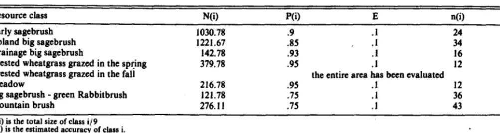
Tabk 1. Singk stage clustering parameters for determinhg sample size.
Resource class N(i) P(i) E n(i) L Early sagebrush 1030.78 .9 .I 24 24 Upland big sagebrush
Drainage big sagebrush
Crested wheatgrass grazed in the spring Crested wheatgrass grazed in the fall
Meadow
Big sagebrush - green Rabbitbrush Mountain brush
N(i) is the total size of class i/9 P(i) is the estimated accuracy of &ss i. E is the estimated accuracy of class i. n(i) is the number of clusters needed, (sample sise).
1221.67 142.78 379.78 216.78 121.78 276.11
L is the actual number of clusters sampled, (actual sample size).
.85
::
34 35
.93 16 15
.95 .I 12 I2
the entire area has heen evaluated
.95 .l 12
.75
:t
:26 3
.75 43 5
allowed in a cluster. This procedure classifies most pixels and can be interpreted and reinterpreted until the classification fits the range vegetation mosaic at an acceptable level as determined by ground sampling. It also eliminates the need for locating homo- geneous training sites since the computer groups like pixels automatically.
was located so accuracy could be assessed. Minimum sample size required for each class (Table 1) was determined using the formula (Todd et al. 1980):
In mixed or guided clustering approach a combination of the where: above 2 approaches is used. A training window, containing some
general vegetation type as determined from field observation, is selected by the analyst to include subtle differences in vegetation ’ patterns that are difficult to identify using either of the above 2
approaches alone. This allows the definition of unique Cband signatures for homogeneous plant communities not readily defined in the unsupervised classification.
n(i) = N(i)p(i)q(i) (N(i) (B*/t*)) + p(ihRi)
n(i) is the number of clusters needed (sample size) N(i) is the total size of class i divided by 9
p(i) is the estimated accuracy of class i E is the allowable error (0.10)
t is the Student’s I statistic at the allowable error and q(i) is L-p(i)
In this study a combination of all 3 of these methods was used to arrive at the final classification map. The supervised approach was used for the hay meadows and the unsupervised and guided cluster- ing approaches were used on the various sagebrush communities.
Accuracy Evaluation
Ground data for evaluation plots were randomly selected on 1:24,000 color infrared aerial photographs using a grid system with each cell being the size of a pixel. These plots were plotted on 1:24,000 scale topographic maps and their vegetation types verified through field observation. Normally, evaluation samples are select- ed from the iandsat classification map to obtain a completely random sample (Todd et al. 1980). In this study random samples were not used because of the variable nature of range vegetation (making it difficult to locate homogeneous evaluation plots). Eco- tones were not sampled since they constitute a source of noise- induced error (Daus 1975) where boundary Landsat pixels will include reflectance information from both plant communities.
The initial estimated accuracies of the different classes (p(i)) were determined by preliminary field checking of easily accessible field plots and calculating the percent correct.
Accuracy was calculated in the form of percent correct in class i and an average classification accuracy calculated from these values (Table 2). Confidence intervals were calculated using the standard Student’s t formula (Table 3). The standard error of the estimate of
p(i) (S.E.(p(i)) was used to calculate confidence intervals using the formula for an even number of sample elements within cluster samples (Cochran 1963);
S.E.(p(i))
q
v!!where: g.B. (p(i)) is the standard error of the estimate p(i). puj IS the percent correct in the jth cluster in class i, p(i) is the percent correct for class i, and
n is the number of clusters in class i.
Results and Discussion
Within each evaluation plot at least 1 3X3 pixel cluster sample
Table 2. Vegetation ckssifiatlon l ccurecy.
The final Landsat classification resulted in 14 spectral classes
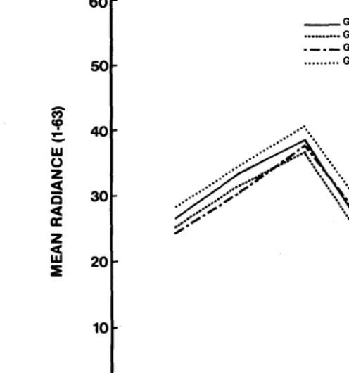
representing 8 range plant communities (Table 4). Spectral signa- tures for the 14 spectral classes are very similar (Fig. 1).Number of ground observations Crested Big wheatgrass sagebrush
Early Upland Drainage grazed in green Mountain
sagebrush bigsage bigsage spring rabbitbrush brush Meadow Number of Landsat observations
Early sagebrush 187 2z 1 2
Upland bigsage 10 5 3 5 Drainage bigsage 8 120 1 2 Crested wheatgrass grazed in spring 19 6 103
Big sagebrush-green rabbitbrush 2 23
Mountain brush 11 35
Meadow 2 103
Total 216 315 135 108’ 27 45 108 Number of unclassified pixels 9 1 1 5
Percent correct 86.6% 74.4% S&2% 95.4% 85.2% 77.8% 95.4%
‘Two pixels fell into the crested wheatgrass grazed in the fall class, which is not represented in this table since the entire class was sampled.
T&k 3. Accuracy -t of LnndMt ch&3inc8on. 60
Percent correct Standard error & confidence of the estimate interval at Vegetation class (%I .05 level
Early sagebrush 2.67 86.6% f 5.51 Upland big sagebrush 4.22 78.4% f 8.57 Drainage big sagebrush 2.17 88.2% f 4.62 Crested wheatgrass grazed in 2.54 95.4% f 5.53
spring
*Big sagebrush- 85.2%
green rabbitbrush
Mountain brush 7.87 77.8% f 20.23
Meadow 2.54 95.4% f 5.75
Crested wheatgrass grazed in fall Entire class was 83% sampled
Mean accuracy of all sample plots
*Inadequate sample for calculation of statistics.
86.4%
The sagebrush classes have progressively higher means across the 4 bands as canopy cover decreases from class to class (Fig. 2). The meadow classes have a characteristic spectral signature for dense green vegetation. The grass classes (Grass 1,2,3,4) have a characteristic green shift in band 6 with Grass 4 being highest in band 6 as expected since it is not grazed until fall and it is on the more moist site, giving it the highest green biomass (Fig. 3). Grass 3 is not grazed until fall either, but has considerable invasion of sagebrush, causing it to fall between Grasses 1 and 2 in band 6. Grasses 1 and 2 are grazed in the spring.
Fig. 1. Mean spectral radiance for each statistical class.
The percentage correctly classified ranged from a high of 95.4% for the sample plots in the crested wheatgrass seedings grazed in the spring and for the meadow class, to a low of 77.7% for the sample plots in the mountain brush vegetation (Table 2). The overall mean classification accuracy for all sample plots was 86.4% (Table 3).
Most of the 14 spectral classes were identified by careful photo interpretation. However, classes such as Bigsage 1 and 2 and Grass 3 and 4, while different on the ground, could only be separated using the computer and spectral space as defined by the Landsat digital data. They were not readily identified on the aerial photographs.
plant vigor. Bigsage 3 was found exclusively in the drainage bot- toms where it has the highest canopy cover and the greatest overall vegetation vigor. Bigsage 2 (medium density) was found either in conjunction with Bigsage 3 along drainage bottoms or in smaller drainages at the base of the mountain range where soils are deep and relatively moist. Bigsage 1 has the lowest canopy cover and is found with greater frequency on shallower soils as one moves eastward from the mountain range.
The big sagebrush types were separated into 3 different big sagebrush spectral classes (Bigsage 1,2, and 3). Bigsages 1 and 2 were combined to form the “upland bigsage” range type because they are extremely difficult to differentiate in the field. Differences among the big sagebrush classes were related to canopy cover and
These 3 big sagebrush classes are generally related to 3 sub- species of big sagebrush found in the area. Bigsage 3 (drainages) is dominated by big sagebrush, Bigsage 2 (intermediate big sagebrush sites) by mountain big sagebrush, and Bigsage 1 (poorest big sagebrush sites) by Wyoming big sagebrush.
Only one spectral class representing the early sagebrush type could be identified. Early sagebrush is relatively homogeneous and consistent on clay hardpan soils of the lower parts of the study area. Early sagebrush areas are referred to as lowsage in the tables and Figure 2.
1
I I I IBAND 4 BAND 5 BAND 6 BAND 7
Tabk 4. Suamwy of statktkal and resource ckmu for the Savd study area.
Statistical class
Lowsage
Bigsage I Bigsage 2
Bigsage 3
Grass I Grass 2
Grass 3 Grass 4
Meadow Meadow 1 Meadow 2 Mountain I Mountain 2
Bigrab
Resource class Pixels Hectares Percent of total area
Early sagebrush 9077 4099 26.3%
Upland big sagebrush 10712 4837 31.0%
Upland big sagebrush
Drainage big sagebrush 1250 564 3.6%
Crested wheatgrass 5878 2654 17.0%
Grazed in the spring
Crested wheatgrass 1174 530 3.4%
grazed in the fall
Meadow 1901 860 5.5%
Mountain brush 2423 1094 7.0%
Big sagebrush-green rabbitbrush 1076 486 3.1%’
Unclassified 1009 496 3.2%
Total 34500 15619 100.00%
_ LOWSAGE . . . SlGSAGEl
.-.-SlGSAGE2
. . . BIGSAGE
60
_ GRASS 1
.._... GRASS 2
.-.-GRASS 3
so . . . GRASS 4
BAND4 BAND5 BAND6 BAND7 BAND 4 BAND 5 BAND 6 BAND 7
Fig. 2. Meon spectral radiance for each sagebrush cleps.
The crested wheatgrass seedings were divided into 4 different spectral classes. Grasses 1 and 2 were grazed heavily in the spring and have considerable bare soil. Grass 3 is confined mostly to one pasture that was grazed only in the fall. It was more vigorous than Grass I or 2. Grass 4, also grazed in the fall, was even more vigorous than Grass 3, because it was located in a moist bottom- land close to a drainage. The 3 meadow spectral classes were grouped together because meadow classification was not the emphasis of the study.
At the base of the mountain range there were 2 mountain brush classes that were also combined to form a single class dominated by a variable mixture of big sagebrush, mountain mahogany (Cerco-
carpus ledifiius), and bitterbrush (Purshia tridentata). A final
range type identified was a mixture of big sagebrush and green rabbitbrush. It is composed of nearly an even mix of big sagebrush and green rabbitbrush (Chrysothamnw viscidiflorus) and is usu- ally found in the lower parts of major drainages.
Some pixels remained unclassified (Table 2). These pixels were either ecotones or areas not large enough to form their own statisti- cal classes such as corrals or small stock watering ponds. Few software packages depict unclassified pixels. However, they are valuable for quickly locating and evaluating areas that do not represent any class and for decreasing misclassification. Because of vegetation heterogeneity, no given range should be classified with- out some unclassified pixels. In this classification 1,009 out of 34,500 or 2.9% of the pixels remain unclassified, a reasonable number for an allotment of this size. This characteristic of the analysis can be extremely valuable in identifying resource classes that may have been overlooked.
The early sagebrush vegetation presented 2 major classification problems. First, a large number (41) of “upland bigsage” pixels (Bigsage I) were included in the early sagebrush class. Field inves- tigation revealed the areas of upland big sagebrush tend to be confused with early sagebrush since they had low canopy cover, a high percentage of bare soil, and recently had received heavy grazing. Second, some early sagebrush (19) pixels were placed in the grass category. These spots were difficult to locate precisely in the field because they are so widely scattered. This classification problem appears on areas where early sagebrush is very sparse and where cheatgrass (Bromus tectorum) and bare soil are common.
630
Fig. 3. Mean spectral rodtoncefor each gross class.
Areas of sparse early sagebrush produce a spectral signature sim- ilar to that of grazed crested wheatgrass (Grass 1 and 2). Also, this misclassification may be caused by a high density of ant mounds 1.5 to 2m in diameter. A large number of mounds and bare soil in early sagebrush stands produces a signature similar to grazed crested wheatgrass.
Mountain brush and upland big sagebrush communities were confused (11 pixels). Mountain brush types occur in patches throughout the upland big sagebrush with no definite transition zone. Field interpretation is difficult and is likely the cause of some classification errors.
Neither the mountain brush or big sagebrush-green rabbitbrush classes were adequately sampled (Table 1). Both plant communi- ties are widely scattered and were often represented by 1 or a very small group of pixels. Sampling was thus extremely difficult and obtaining an adequate sample was impossible. Percentage correct results for these 2 classes may be misleading. Their scattered distri- bution made it impossible to conclude whether misclassification errors were due mostly to the scattered and spotty nature of the stands or whether they were not spectrally distinct.
Using the PIXSYS software with Landsat digital data and guided clustering techniques, 3 different canopy cover classes of big sagebrush and 2 different sagebrush communities, early sage- brush and big sagebrush, were separated. On crested wheatgrass seedings, those grazed in the spring are readily separable from those grazed in the fall. Crested wheatgrass grazed in the spring was not separable from cheatgrass-invaded areas in early sage- brush vegetation.
The spectral differences among range plant communities as derived from Landsat classifications are often very small. Differ- ences between spectral classes that represent these communities tend to approach the noise level of the Landsat data. Because of the lack of relatively large homogeneous evaluation sites, it was impos- sible to conclude whether mountain brush and big sagebrush-green rabbitbrush were always distinguishable from other sagebrush communities at the study site.
A difficult problem common to this and most Landsat studies is the requirement for adequate ground data. Other techniques for separating vegetation signatures from bare ground signatures such as band ratioing (Tucker 1977) deserve investigation on desert
shrublands.
Landsat digitized classification and mapping has potential for use in rangeland vegetation inventory. Studies such as this, Max- well’s (1976), and Bonner and Morgart’s (1980) show that Landsat is a presently available data source that can be used to collect at least general baseline data for range inventories. With continued research into the use of digital Landsat data for automated range- land inventories, combined with digitized aerial photography and geographic information (elevation, slope, soils, etc.), range trend and productivity may eventually be monitored economically and on a regular basis.
Literature Cited
Banner,
William J., and John Morgart. 19M). Landsat: A Sampling Frame For Arid Land Inventories. Proceedings Arid Land Resource Inven- tories: Developing Cost-Efftcicnt Methods. An International Workshop. Nov.-Dec. LaPax, Mexico. p. 23@239.Cochran, W.T. 1963. Sampling techniques, 2nd edition. John Wiley and Sons Inc., N.Y.
Daus, SJ. 1975. Utilization of automated data analysis techniques for Landsat-based range resource evaluations. In: Spacecraft and aircraft remote sensing for integrated unit resource inventory and analysis in
northeastern California and northeastern Nevada. R.N. Colwell (ed.) BLM Final Rep. No. 525004X4-208(N).
Everitt, J.H.,
A.J.
Richardson, AM. Cerbennan,C.L. Wiegand,andM.A. Ala& 1979. Landsat- data for inventorying rangelands in south Texas. Proc. 1979 Machine Processing of Remotely Sensed Data Symposium. 132-141.Eve&t, J.H., Ad. Richardson, and C.L. W&and. 1981. Inventory of semi-arid rangelands in South Texas with Landsat data. Proc. 1981 Machine Processing of Remotely Sensed Data Symp. Purdue Univ. p. 404-415.
Maxwell, E.L. 1976. A remote rangeland analysis system. J. Range Manage. 2956-7.
Rohde, W.C. 1978. Digital image analysis techniques required for natural resource inventories. AFIPS Conference Proceedings. Vol. 47. USDI Geological Survey, EROS Data Center, Sioux Falls, S.D.
Todd, W.J., D.G. Gebring, J.F. Haman. 1980. Landsat wildland mapping accuracy. Photogrammetric Engineering and Remote Sensing 6509-520.
Tucker, C.J. 1977. Use of near infrared/red radiance ratios for estimating vegetation biomass and physiological status. NASA/GSFL preprint X-923-77-183.
Tueller, P.T., F.R. Honey, and IJ. Tapley. 1978. Landsat and photo- grahic remote sensing for arid land applications in Australia. Proc. 12th Intern. Symp. of Remote Sensing. Vol. 3. p. 2177-2191.
CHANGE OF ADDRESS notices should be sent to the Managing Editor, 2760 West Fifth Ave., Denver, Colo. 80204, no later than the first day of the month of issue. Copies lost due to change ot address cannot be replaced unless adequate notice is given. To assure uninterrupted service, provide your local postmaster with a Change of Address Order (POD Form 3575) indicating thereon to guarantee forwarding postage for second-class mail.