CHARACTERISTIC BASIS FUNCTION METHOD FOR ITERATION-FREE SOLUTION OF LARGE METHOD OF MOMENTS PROBLEMS
R. Mittra and K. Du
EMC Laboratory Penn State University
319 EE East, University Park, PA 16802, USA
1. INTRODUCTION
We observe that there is a rapidly growing trend in Computational Electromagnetics (CEM) that is significantly impacting the computing landscape, namely the use of highly parallel computers to address large and complex problems. It is well known, however, that with the exception of the FDTD-based codes that are “embarrassingly parallel,” not all computer codes scale equally well on these platforms. The CBMoM (Characteristic Basis Method of Moments) code, which is based on CBFM, is another exception, since, unlike the conventional MoM codes, it also can be parallelized efficiently. This implies that even problems characterized by a large number of degrees of freedom (DoFs) can be solved by using direct methods as opposed to iteration; this is a unique feature of CBMoM that is not present in conventional MoM codes.
The organization of the paper is as follows. In Section 2 we present the details of CBFM for microstrip circuits to lay the foundations of the method. We show how we can use the concepts of domain decomposition and high-level or macro basis functions to significantly reduce the size of the MoM matrix, which can then be solved directly, without relying on iteration. This feature, as well as the fact that, unlike the FMM, CBFM is not kernel-dependent, makes the CBMoM somewhat unique — as well as highly desirable — as an approach for handling large problems. Next, in Section 3, we describe the version of CBFM suitable for scattering problems that is based on the same basic concepts outlined in Section 2. Finally, we describe some recent developments in CBFM in Section 4 and present some summary conclusions in Section 5.
2. CBFM FOR MICROSTRIP CIRCUITS AND PRINTED ARRAYANTENNA PROBLEMS
contribution to the total solution, only a finite number of mutual-coupling currents, referred to as the “secondary” bases in CBFM, need to be retained in the solution process. Consequently, the total number of characteristic basis (CB) currents, which correspond to the effective degree of freedom (DoF) for the system, is typically orders of magnitude less than in the conventional MoM formulation. This, in turn, leads to a reduced matrix, which is much smaller than the original MoM matrix, even though it captures all the interactions between different parts of the circuit without compromising the accuracy.
The CBFM begins by dividing the original problem geometry into sub-blocks, such that the MoM matrix for each sub-block can be easily computed and solved on a single personal computer. Next, it generates the characteristic bases (CBs) that are the induced currents on one of the sub-blocks by using certain types of excitations, as explained below. The CB is referred to either a “primary” or a “secondary”, depending on the type of excitation. Finally, we form the reduced matrix equation by using the Galerkin procedure. Solving the reduced system gives the weights of the characteristic bases such that their weighted summation represents the desired current on the original circuit.
To get into further details of the formulation, we start with the conventional MoM procedure, whereby the mixed potential integral equation is discretized into a matrix equation:
Z·I=V. (1)
where Z denotes the conventional MoM impedance matrix; I is the unknown current vector; and, V is the excitation voltage vector. As explained earlier, the “finite DoF” premise of the algorithm essentially asserts that the desired solutionI of (1) can be represented as:
I=N
i=1ciIi, (2)
whereIi (i= 1, . . . , N) represent the characteristic basis currents, and
ci denotes the “magnitudes” or weights of these currents. Methods of finding Ii and ci will be prescribed later. Note that each Ii would have non-zero entries only at the positions belonging to a sub-block and its terminals. WhenIi is normalized, the value ofci indicates the physical significance of the i-th CB and, hence, the “importance” of certain coupling effects between the sub-circuits. This observation is useful in determiningN, the total number of characteristic bases that would yield an accurate solution to the problem at hand.
source applied at the terminals of the sub-blocks. These terminals are either the excitation ports of the original problem, or artificial edges introduced as a result of the division of the original geometry. Once all of the primary CBs have been computed, we assign the primary CB on one of the sub-block as the excitation and compute the secondary currents induced on the other sub-blocks. Likewise, by using a secondary CB as the excitation, we can obtain the tertiary CBs, if we so desire.
Let us consider a simple case where the original problem is divided into two sub-blocks (AandB), eachof whichhas two terminals (1 and 2). For this two-block problem, the system matrix Z in (1) can be written as:
Z=
ZAA ZAB ZBA ZBB
. (3)
Here the sub-matrix ZAA is the MoM matrix for sub-block A; ZBB
corresponds to sub-block B;ZAB represents the coupling between the sub-blocks Aand B. The 4 primary bases can be obtained by solving
ZAA·IA(1,or 2) = VA(1,or 2), (4)
orZBB·IB(1,or 2) = VB(1,or 2). (5)
The subscripts “(1)” and “(2)” appearing above indicate the values correspond to local excitations at the two terminals (“ports”). The secondary basis on sub-block B can be derived by solving for the IB
in (6) below:
ZBB·IB =−ZBA·IA, (6)
where IA appearing in the right hand side (RHS) of (6) is taken as the primary CB supported by sub-blockA(solution of (4)). Similarly, the secondary basis whose support is sub-block A can be computed by using the primary CB on sub-blockB as the excitation. Naturally, the solutions of (4), (5) or (6) would have to be padded with zeros at appropriate locations so that all the primary and secondary bases would have the same dimensions, as in (2).
Our next task is to calculate the weightsci in (2) for a given RHS corresponding to the excitation of the one of the ports in the original problem. Towards this end, we apply the Galerkin procedure once more, and employ the CBs calculated earlier as the testing functions. This leads us to the following matrix equation for the “reduced current vector”IR whose entries are theci’s:
Here ZR is anN ×N reduced system matrix given by
ZR≡BTZRB, (8)
B is a matrix withN columns defined by
B= [I1 I2 . . . IN]. (9)
The superscript “T” in the above equations denotes a matrix transpose. Several methods for fast matrix-vector multiplication that are available in the literature can be used to efficiently compute the coefficients in (7), if desired. As mentioned before, substituting the solution of Eq. (7) in to the expression in Eq. (2) gives the induced current. The other circuit or antenna parameters can be obtained by following the conventional post-processing procedure.
We next present some numerical examples to demonstrate the application of the CBFM to microwave circuit [10] and antenna problems [11].
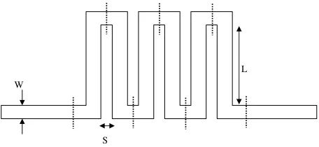
2.1. Meander Line Filter
Figure 1 shows a meander line filter printed on a dielectric slab with a ground plane. The dielectric constant is εr = 2.43, the thickness is 0.49 mm, while the other length parameters as indicated in the figure are: W = 1.41 mm, S = 2.82 mm and L = 29.61 mm. We apply the MoM in the conventional way, and discretize the geometry into 624 rectangular cells corresponding to 1039 unknowns using rooftop basis functions. The CBFM is implemented for this geometry over the frequency range of 9 to 11.5 GHz, the computational time is determined, and the accuracy of the computed S-parameters is evaluated. We begin by segmenting the geometry into 8 sub-blocks
W
S
L
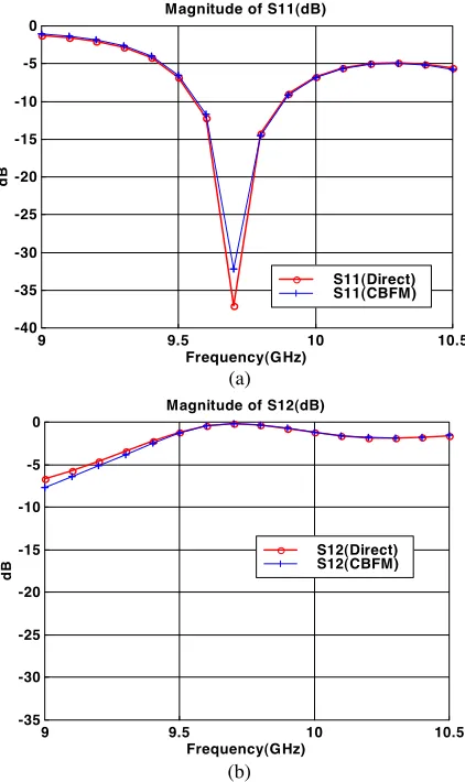
as shown in Fig. 1. We next apply the CBFM in two different schemes to compute the S-parameters. In the first scheme, we include no secondary CBs. The S-parameters, thus obtained, are compared with those from the direct solution (see Fig. 2). Except for minor differences near the resonance and at frequencies below 9.5 GHz, the two sets of
S-parameters matchwell witheachother. This can be attributed to fact that the primary CBs constitute the main component of the induced current and that there exists only a relatively small level of field coupling between the sub-blocks. In the second scheme, we include
9 9.5 10 10.5
-40 -35 -30 -25 -20 -15 -10 -5 0
Magnitude of S11(dB)
Frequency(GHz)
dB
S11(Direct) S11(CBFM)
(a)
9 9.5 10 10.5
-35 -30 -25 -20 -15 -10 -5 0
Magnitude of S12(dB)
Frequency(GHz)
dB
S12(Direct) S12(CBFM)
(b)
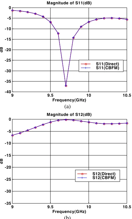
all of the secondary CBs, leading to a total of 128 CBs — almost an order of magnitude smaller than the original number of unknowns in the conventional MoM. The S-parameters calculated from the second approachare compared withthose obtained from the direct solution in Fig. 3. The two sets of results are indistinguishable from each other. This is not unexpected since we have now included all the first-order mutual coupling effects, which is sufficient for the purpose of evaluating theS-parameters.
9 9.5 10 10.5
-40 -35 -30 -25 -20 -15 -10 -5 0
Magnitude of S11(dB)
Frequency(GHz)
dB
S11(Direct) S11(CBFM)
(a)
9 9.5 10 10.5
-35 -30 -25 -20 -15 -10 -5 0
Magnitude of S12(dB)
Frequency(GHz)
dB
S12(Direct) S12(CBFM)
(b)
Figure 3. Comparison ofS-parameters of the meander line calculated by using the CBFM and the direct solver. Primary CBFs and all of the secondary CBFs were used. (a) Magnitude of S11. (b) Magnitude
2.2. Two-stage Amplifier
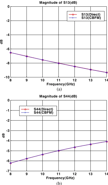
For the next example, we present the simulation results of a two-stage amplifier circuit shown in Fig. 4. The circuit is printed on a 0.254 mm thick Alumina (εr= 9.8) substrate witha ground plane on the bottom. This problem requires 1819 unknowns when the conventional Method of Moments is used. To apply the CBFM, the geometry is segmented into 7 sub-blocks as shown in Fig. 4. We first ignore all the lumped circuit components (capacitors, resistors and active transistors) and simulate the S-parameters of the resulting multi-port circuit over the frequency band of 8 to 14 GHz. We plot, in Fig. 5, a few selected S -parameters, calculated via the CBFM as well as by using the direct method. It is evident that theS-parameters obtained from the CBFM are in good agreement with those derived via the direct solution. We then simulate the performance of the entire system by combining the
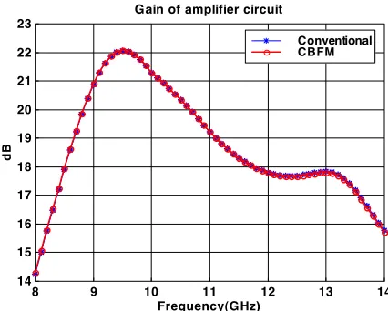
S-parameters of the multiport circuit with the lumped components in a circuit simulator. The gain of the amplifier circuit thus obtained is shown in Fig. 6. We note that the gain plot also shows a very good agreement between the CBFM and direct solutions. For this problem, a total of 96 CBs are needed throughout the entire frequency band. The time required to obtain the S-parameters at the 61 frequency points is 132 seconds when using the CBFM, in contrast to the 968 seconds required by the direct solution.
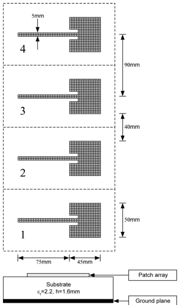
2.3. 4×1 Patch Array Antenna
Next we consider the example of a 4×1 patcharray fed by microstrip lines as shown in Fig. 7. Each of the rectangular patches is 50 mm long and 45 mm wide. The 50 Ω feed-line has a width of 5 mm and a
8 9 10 11 12 13 14 -10
-8 -6 -4 -2 0
Magnitude of S13(dB)
Frequency(GHz)
dB
S13(Direct) S13(CBFM)
(a)
8 9 10 11 12 13 14
-7 -6 -5 -4 -3 -2 -1 0
Magnitude of S44(dB)
Frequency(GHz)
dB
S44(Direct) S44(CBFM)
(b)
Figure 5. Comparison of theS-parameters of the passive components of a two-stage amplifier circuit computed by the CBFM using the primary and the secondary CBFs with thresholding, and the direct method. (a) Magnitude ofS13. (b) Magnitude ofS44.
8 9 10 11 12 13 14 14
15 16 17 18 19 20 21 22 23
Gain of amplifier circuit
Frequency(GHz)
dB
Conventional CBFM
Figure 6. Comparison of the gain of the entire two-stage amplifier circuit computed by using the CBFM and the conventional method.
block when applying the CBFM. A conventional approach to modeling this antenna requires 2.932 unknowns using rectangular rooftop basis functions. Each of the four blocks has 733 unknowns. The array has an expected resonant frequency slightly above 2 GHz, and the proposed CBFM is implemented over a frequency range of 1.8 to 2.7 GHz.
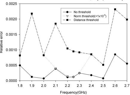
Three different methods are used for generation of the CBs for eachblock, witha view to comparing their performance. For the first case, all of the secondary CBs are constructed with no thresholding and, hence, 3 secondary CBs are generated for each block, leading to a total of 16 CBs (including the primary ones). For the second case, the number of secondary CBs is reduced by applying a threshold level of 10−5 to the relative norm Isecondary/Iprimary. The number of secondary CBs is allowed to vary as a function of the frequency. Note that a larger number of secondary CBs are needed near the resonance frequency, owing to stronger mutual couplings between the elements. Finally, we also generate the secondary CBs based on the distance criterion between the blocks, by retaining only the secondary CBs that are associated with the surrounding blocks in all directions. The resulting number of the CBs is now 10 and it remains unchanged over the frequency band.
out the LU factorization only once for the first block and use it later, repeatedly, to avoid redundant computation. The number of the CBs is plotted in Fig. 8 as a function of the frequency for the three cases.
The current coefficients obtained for these cases are compared to those obtained from the direct solution. The error for the current
coefficients is defined aseI ≡
n |
ICBF M
n −Indirect|
2
n |
Idirect
n |
2
.
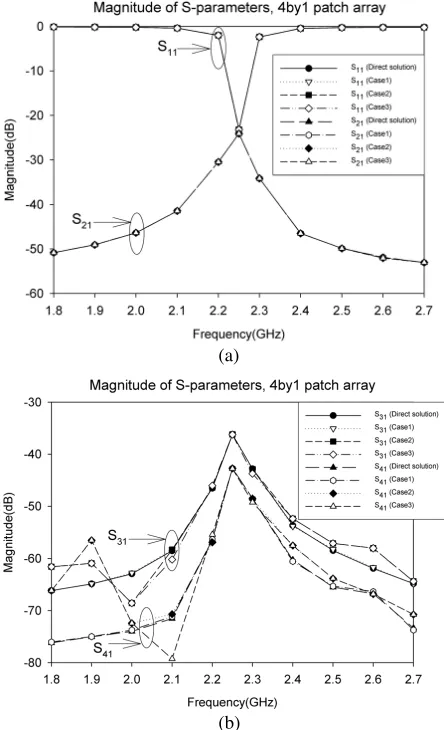
This error norm and theS-parameters for the three cases are compared in Figs. 9 and 10, respectively. We observe that except for minor differences in theS31 and S41 parameters at off-resonance frequencies
— where their levels are very small (below −50 dB) — all of the S -parameters match well with those predicted by the direct solution. The radiation patterns for the third case, which utilized a distance threshold, are compared to those of the direct solution in Fig. 11.
Figure 8. The number of the CBFs as functions of the frequency for the 4×1 patcharray fed by microstrip lines.
Figure 9. Relative error in the current coefficients for the 4×1 patch array fed by microstrip lines (port 1 active).
3. CBFM FOR SCATTERING PROBLEMS
As we saw in the last section, the basic steps in CBFM entail the generation of primary and secondary basis functions for the representation of the induced currents and the solution of the reduced matrix to derive the desired unknown currents. Although we could follow exactly the same basic procedure for the scattering problems as
(b) (a)
Figure 10. Comparison of theS-parameters for the 4×1 patcharray fed by microstrip lines: (a) magnitudes ofS11andS21; (b) magnitudes
(a)
(b)
Figure 11. Comparison of the radiation patterns at 2.25 GHz for the 4×1 patcharray fed by microstrip lines: (a) θ = 0◦ cut; and (b)
φ= 90◦ cut.
the same reduced matrix, to derive the solutions for different incident angles by simply changing the RHS of the reduced matrix equation.
Plane Wave Spectrum on Block
Individual Block
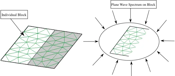
Figure 12. Spectrum of plane waves incident on a single block.
As before, we begin by dividing the geometry of the object to be analyzed into blocks, for instance M in number. Next, we derive the primary characteristic basis functions by illuminating the isolated blocks withplane waves, say NP W S in number (see Fig. 12), which impinge upon the object at intervals of θand φ, say every 20 degrees, for two orthogonal polarizations. We can be flexible in choosing the number of these incident waves, and can also include a part of the invisible range of the spectrum — if desired — since the SVD will downselect the number of basis functions to remove the redundancy and will retain only as many as needed to represent the unknown current witha certain degree of accuracy, determined by the level of the SVD threshold we set. In addition, the decomposition of the object into blocks is also somewhat arbitrary, and there is no limitation on the number and size of the blocks. The upper size is bounded by the available RAM needed for the unknowns in the self-blocks that are solved to generate the CBs. Typically, the block size ranges from a few hundred to a few thousand sub-domain type of unknowns. As pointed out earlier, the advantages of following this procedure is that it enables us to solve for multiple excitations using the same reduced matrix with a significant time-saving, since only the RHS of the reduced system needs to be computed for a new excitation.
For the sake of illustration, we consider a thin plate which is divided into 25 blocks, shown in Fig. 13. Although, in general, the blocks can have different sizes, we assume that they have approximately the same dimensionNb in terms of number of unknowns.
Z
Figure 13. Geometry of a PEC plate divided into 25 blocks. Extended blocks are represented in dashed lines.
except when the boundaries are free edges, to avoid a singular behavior in the current distribution within the original block introduced by the truncation that creates fictitious edges. Each of the M extended blocks are represented by the Nbe ×Nbe self-impedance matrix Zii, where i = 1,2, . . . , M, and Nbe is the number of unknowns in the extended blocks. The matrix Zii is extracted from the original MoM matrix by using a matrix segmentation procedure. The concept of MoM matrix segmentation is illustrated in Fig. 14, where the extended and individual blocks are shown by dotted and solid lines, respectively. The self-impedance matrix is then used to generate the primary CBs induced on a given block by exciting the block with a set ofwindowed plane waves, impinging upon the object with different incident angles (θ, φ), and withtwo linear different polarizations. The windowing is used to reduce the effect of truncation employed in the process of domain decomposition.
Let Nθ and Nφ indicate the number of samples in elevation and azimuth(θ and φ) respectively. This results in a total of NP W S =
NφNθ plane wave excitations, which are arranged in a matrix VP W Sii , whose size isNβε·NφNθ. After exciting the block,NφNθ primary CBs are determined for eachblock by solving the following linear system of equations:
Zextii ·JCBF sii =ViiP W S, (10)
Zext Zext
Figure 14. MoM matrix segmentation procedure. Individual and extended blocks are shown in solid and dotted line, respectively.
the extension region, so that the resulting CBs are now confined within the original block, and their size is now reduced toNb×NφNθ. Even though the size N of the complete MoM matrix may be very large if the original structure is large in terms of the wavelength, the dimension of each block can still be kept to a manageable level and, hence, the linear system (10) can be solved by using an LU decomposition. This factorization is highly desirable since we have to solve (10)NφNθtimes, once for eachincident plane wave, to compute the complete set of primary basis functions.
Typically, the number of plane waves we use to generate the CBs would exceed the number of degrees of freedom (DoFs) associated with the block, and it is desirable to remove the redundancy in the basis functions by applying a Singular Value Decomposition (SVD) procedure, and thresholdingJii. This is done by expressing the latter as:
JCBF sii =UDVt, i= 1,2, . . . , M, (11)
process of eliminating the post-SVD CBs is important to reduce their redundancy and, consequently, improve the condition number of the reduced matrix. For the sake of simplicity, we assume that all of the blocks contain the same number K of CBs after SVD, where K is always smaller thanNφNθ.
It is worthwhile mentioning that the “new” primaries have all the desired characteristics of wavelets; however, in contrast to the wavelets, they are tailored to the geometry of the object. Thus, unlike the wavelets, the post-SVD CBs can be used for an arbitrary three-dimensional object, without any restrictions.
Following the procedure described above, we construct KM
primary basis functions, K for eachof the M blocks. The solution to the entire problem is then expressed as a linear combination of the CBs as follows:
J = K
k=1
α(1)k
J(1)k
[0] .. . [0] + K k=1
α(2)k
[0]
J(2)k
.. . [0] +. . .+ K k=1
α(kM)
[0] [0] .. .
J(kM)
(12)
where α(km), for m = 1,2, . . . , M, are the unknown expansion
coefficients to be determined by using the reduced matrix, andJ(km)is thekthCB of blockm, fork= 1,2, . . . K. The final step is to generate the reducedKM ×KM MoM matrix for the KM unknown complex coefficients αk by performing the inner product on Eq. (1) onceJ has been expressed as in (12).
The reduced coefficient matrix has the form:
[Z]KM×KM=
Jt
11Z11J11
Jt
11Z12J22
. . . Jt
11Z1MJM M
Jt
22Z21J11
Jt
22Z22J22
. . . Jt
22Z1MJM M
..
. ... . .. ...
JtM MZM1J11 JtM MZM2J22
. . . JtM MZM MJM M
, (13)
of the inner product entries in the above matrix results in a sub-matrix of sizeK×K, and the MoM matrix reduction involves M K2 complex matrix-vector products. The time advantage of reducing number of primaries, via the SVD approach, is shown in Table 1, which presents the time performance results for different SVD thresholds.
After performing the necessary operations indicated in (13), the original MoM matrix in (10) is reduced to a smaller one. The induced surface current distribution for the entire structure can now be obtained by substituting the values ofα in (12). Once the current density distribution has been derived, the electrical parameters such as RCS, scattered field, etc., can be computed in the usual manner.
The most computationally intensive part of the proposed method is associated with the generation of the primary CBs and the matrix reduction procedure. However, the latter task can be speeded up by observing that the following relationship holds:
JtmmZmnJnn
=JtmmZmnJnn t
=JtnnZnmJmm
, (14)
since Ztmn = Znm. Taking advantage of this, the complexity in computing (13) can be reduced by a factor of two, since we need only generate the upper or lower triangular parts of the reduced matrix.
Generation of CBs is one of the time-consuming and memory-demanding tasks. It requires the filling the self-impedance matrixZii for the extended block and its factorization in an LU form. Since the CBs are independent of the incident angles, this factorization needs to be performed only once, and the resulting primaries can be reused for multiple incident angle directions. This implies that the final reduced matrix (5) is independent of the excitation, and this fact enables us to solve a problem involving multiple excitations by only solving the reduced system for the new r.h.s. (excitation). Moreover, we can store the reduced matrix on the hard disk and reuse it whenever we need to analyze a new excitation. Furthermore, if the geometry within a particular block is modified, only the CBs belonging to this block need to be recomputed.
The technique described above realizes a saving in the CPU running time and RAM requirement withrespect to a conventional MoM technique. The memory requirement is now proportional to the square of the self impedance matrix of the extended block, and this is different from that in the conventional MoM where the storage requirement is related to the square of the dimension of the entire impedance matrix. Moreover, we realize a consistent saving in the execution time, which reduces toO(M(Nbe)3) instead of O(N3).
3.1. Plane Wave Scattering by a 4λ Radius PEC Sphere
To validate the accuracy of the method we will compare the CBFM solution with the analytical one for a PEC sphere of radius 4λ, at a frequency of 300 MHz. The object is excited by a normally incident (θ = 0◦, φ = 0◦) theta-polarized plane wave. The discretization is carried out by using triangular patches with a mean edge length of 0.1λ, resulting in a problem with85155 unknowns. The geometry is divided into 16 blocks withan average size of 8000 unknowns. Eachblock is extended by ∆ = 0.4λin all directions, and analyzed for a spectrum of plane waves incident from 0◦ ≤θ < 180◦ and 0◦ ≤φ <360◦, with
Nθ =Nφ= 20. This results in a total of 800 CBs but, after SVD, only 310 are retained on eachblock. The 85155×85155 MoM matrix is then reduced to only 4925×4925, which is solved directly.
At this point we mention that the construction of the CBs can be speeded up, withlittle loss of accuracy, by using a sparsified version of the self-blocks — that retain only the near-region interactions — rather than working with the full versions of these blocks. It is possible to work with the sparsified matrices, because they are used to generate only the basis functions and not yet the solution. Thus, so long as the basis functions span the solution space, they need not strictly be solutions of the original self-blocks. To validate this concept, we have analyzed the problem at hand by using both dense and sparse matrix approaches. The use of the latter allows us to reduce the computational cost by a factor of approximately 4. The bi-static E- and H-plane RCS results are presented in Figs. 15(a) and 15(b), respectively, using the dense and sparse approaches, as well as the MIE series, and they show an excellent agreement for all scattering directions, including the grazing angles.
3.2. Parallel CBFM Applied to the Scattering of a 4λPEC Cube
0 10 20 30 40 50
Sparse Approach
CBMoM
Mie's Solution
0 30 60 90 120 150 180
Bis
ta
tic RCS (dBSm,
φ
=90)
Theta (Degree)
(a)
15 20 25 30 35 40 45 50
S parse A pp roach
C B M oM
M IE
0 30 60 90 120 150 180
Bist
atic RCS
(dBSm,
φ=
0)
T h eta (D e gree )
(b)
Figure 15. RCS of 4λ radius PEC sphere at 0.3 GHz: (a) E-plane; (b)H-plane.
0 0.2 0.4 0.6 0.8 1
100
Matrix Reduction CBFs Generation
Total Computation Time
N
o
rm
a
liz
e
d
C
P
U
T
im
e
Number of Processors
1 10
Figure 16. Normalized CPU times of the parallellized CBMoM code.
-24 -16 -8 0 8 16 24 32
0 50 100 150 200 250 300 350
CBMoM
Parallel CBMoM
Bista
ti
c
RC
S (d
Bs)
Theta (Degree)
Figure 17. Bistatic RCS of a scattering problem by a PEC 4λ side cube at 0.6 GHz, plane (φ= 90◦).
4. SOME RECENT DEVELOPMENTS IN CBFM
to mitigate the effects of truncation introduced during the process of domain decomposition of the original object. Recently [16], it has been demonstrated that by stretching the RWG (or rooftop) basis functions near the edges, it is possible to push the edge effects further out, so that their presence inside the block is minimal. The advantage of using this approach is that the number of unknowns to be solved for in the self-blocks is not increased, as it is when the block is extended by ∆. For smooth bodies, without free edges, there is even a simpler approach that works well for the generation of the CBs. In this method [13], we simply use the Physical Optics (PO) solutions for different plane wave incident fields as the primaries, thereby eliminating the artificial edge effects entirely in the process. The method has also been extended to handle cases where the scatter has free edges, the edge effects are therefore physical, and must be accounted for to generate accurate solutions.
Next, we turn to one of the computationally intensive steps in CBFM, namely the matrix-vector multiplication, required in the process of generating the reduced matrix. We can speed up this step by several ways, namely by: (i) using the FMM approach[14]; (ii) implementing the Adaptive Cross Approximation (ACA) algorithm [15]; or, (iii) employing a newly-developed interpolation approach [17]. We should mention that neither the ACA, nor the interpolation approaches are “kernel-dependent,” and, hence, may be preferable to the FMM for general situations.
Yet another time-saving technique [18] entails the use of multi-level SVD. In this method, we work with a partial range of incident angles at a time, rather than with the entire range of 360 degrees. This, in turn, enables us to work withsmaller size matrices at a time, and thereby results in time-saving when computing the SVDs.
Next, we mention the application of CBFM to locally-modified problems that are handled very efficiently by using this method. This is because we specify that the region that is to be modified locally is to be contained entirely within a single block, say block-1. In this way, we can bypass the CB generation anew in the other blocks when the geometry of block-1 is altered, and derive the CBs in the other blocks only once and for all. We can also limit the generation of the entries for the mutual interactions between the unmodified blocks in the reduced matrix to only once, since they do not change when block-1 is modified. This is a unique feature of the CBFM, not available in the iterative techniques for solving large problems.
localizing the problem, and derive the aperture field distribution. Next, we close the aperture with equivalent currents backed by a PEC. This move enables us to replace the original problem, that of an aperture in an object, with a closed-body problem that has an equivalent magnetic current located on its surface where the aperture was located in the original geometry. To solve this equivalent scattering problem, we need only to modify the RHS, in a way such that it now comprises two sources — the first one being the original plane wave source, while the other is the field radiated by the equivalent current in free space. The CBFM approach itself remains essentially unchanged, except for the fact that now we not only use the plane waves, but also the equivalent current sources to construct the CBs.
Finally, we mention that the CBFM is currently can be generalized to handle dielectric bodies, as well as dielectric-coated PEC objects, by following the same general procedure as outlined above.
5. CONCLUSION AND FUTURE WORK
In this paper we have briefly reviewed the basic concepts of the Characteristic Basis Function Method and have demonstrated how it can be applied to a variety of problems — bothguided-wave and scattering types. Although the general concepts of domain decomposition (DD) have been well known, previous methods relied heavily upon iteration to solve large problems, often using a Jacobi-type algorithm, which is often fraught with convergence problems. The CBFM presents a systematic approach to solving large problems, without the use of iteration, by deriving a reduced matrix whose rank is typically an order of magnitude smaller than that of the original MoM matrix of the scatterer. (However, thought not discussed here, we point out that further reduction can be achieved by using multilevel CBFM). This tactic enables us to solve multiple RHS much more efficiently than when using iterative approaches. Other benefits include efficient solution of locally-modified problems, and frequency sweeping by re-using the basis functions that have been generated for the highest frequency in the range of interest.
ACKNOWLEDGMENT
The authors wish to thank Soonjae Kwon, V. V. S. Prakash and Junho Yeo, all of whom are former members of the EMC laboratory at the Penn State University, for their help and contributions to the text of this article. Special acknowledgements are due to the University of Pisa team, comprising of Eugenio Lucente, Gianni Tiberi, Agostino Monorchio and other former students there, the results of whose research works during the last five years have been extensively used in this paper. Collaboration with Jaime Laviada and his colleagues at the University of Ovieda in Spain, and Carlos Delgado and Felipe Catedra of the University of Alcala, also in Spain, are gratefully acknowledged.
REFERENCES
1. Coifman, R., V. Roklin, and S. Wandzura, “The fast multipole method for the wave equation: A pedestrian prescription,” IEEE Antennas and Propag. Mag., Vol. 35, 7–12, Jun. 1993.
2. Song, J., C. Lu, and W. C. Chew, “Multilevel fast multipole algorithm for electromagnetic scattering by large complex objects,” IEEE Trans. Antennas Propagat., Vol. 45, 1488–1493, Oct. 1997.
3. Michielssen, E. and A. Boag, “Multilevel evaluation of electro-magnetic fields for the rapid solution of scattering problems,” Mi-crowave and Optical Technology Letters, Vol. 7, 790–795, Dec. 5, 1994.
4. Canning, F. X., “Solution of IML form of moment method problems in 5 iterations,” Radio Sci., Vol. 30, No. 5, 1371–1384, Sept./Oct. 1995.
5. Rao, S. M., D. R. Wilton, and A. W. Glisson, “Electromagnetic scattering by surfaces of arbitrary shape,”IEEE Trans. Antennas Propagat., Vol. 30, 409–412, May 1982.
6. Thiele, G. A. and G. A. Newhouse, “A hybrid technique for combining moment methods with the geometrical theory of diffraction,” IEEE Trans. Antennas Propagat., Vol. 23, 551–558, Jul. 1975.
7. Volakis, J. L., A. Chatterjee, and L. C. Kempel, Finite Element Method for Electromagnetics: Antennas, Microwave Circuits, and Scattering Applications, IEEE Press, New York, 1998.
9. Prakash, V. V. S. and R. Mittra, “Characteristic Basis Function Method: A new technique for efficient solution of Method of Moments matrix equation,” Microwave and Optical Technology Letters, Vol. 36, No. 2, 95–100, Jan. 2003.
10. Kwon, S. J., K. Du, and R. Mittra, “Characteristic Basis Function Method: A numerically efficient technique for analyzing microwave and RF circuits,” Microwave and Optical Technology Letters, Vol. 38, No. 6, 444–448, Sept. 2003.
11. Yeo, J., V. V. S. Prakash, and R. Mittra, “Efficient analysis of a class of microstrip antennas using the Characteristic Basis Function Method (CBFM),” Microwave and Optical Technology Letters, Vol. 39, No. 6, 456–464, Dec. 2003.
12. Suter, E. and J. R. Mosig, “A subdomain multilevel approachfor the efficient MoM analysis of large planar antennas,” Microwave and Optical Technology Letters, Vol. 26, No. 4, 270–277, Aug. 2000.
13. Catedra, F., R. Mittra, et al., “Accurate representation of the edge behavior of current when using PO-derived characteristic basis functions,” Submitted for publication on Antennas and Wireless Propagation Letters, Manuscript# AWPL 0307, 2007.
14. Garcia, E., C. Delgado, F. S. De Adana, and R. Mittra, “Devel-opment of an efficient rigorous technique based on the combina-tion of CBFM and MLFMA to solve very large electromagnetic problems,” Electromagnetics in Advanced Applications, ICEAA, 579–582, Sept. 17–21, 2007.
15. Maaskant, R., R. Mittra, and A. G. Tijhuis, “Fast solution of large-scale antenna problems using the Characteristic Basis Func-tion Method and the adaptive cross approximaFunc-tion algorithm,” Submitted for publication onIEEE Transactions on Antenna and Propagation.
16. Laviada, J., M. R. Pino, F. Las-Heras, and R. Mittra, “Mitigation of the truncation problem in the Characteristic Basis Function Method via a novel cell-stretching approach,” To appear inIEEE Antennas and Propagation and URSI Meeting, San Diego, CA, Jul. 5–8, 2008.
17. Laviada, J., M. R. Pino, F. Las-Heras, and R. Mittra, “Efficient calculation of the reduced matrix in the Characteristic Basis Functions Method,” To appear in IEEE Antennas and Propagation and URSI Meeting, San Diego, CA, Jul. 5–8, 2008. 18. Delgado, C., E. Garc´ıa, F. C´atedra, and R. Mittra, “Hierarchical
Antennas and Propagation and URSI Meeting, San Diego, CA, Jul. 5–8, 2008.
19. Tiberi1, G., E. Lucente1, A. Monorchio1, G. Manara1, and R. Mittra, “A characteristic Basis Function Method (CBFM) for analyzing the EM scattering by large structures having slots,” To appear in IEEE Antennas and Propagation and URSI Meeting, San Diego, CA, Jul. 5–8, 2008.
20. Ozgun, O., R. Mittra, and M. Kuzuoglu, “Characteristic Basis Finite Element Method (CBFEM) — A non-iterative domain decomposition finite element algorithm for solving electromagnetic scattering problems,” To appear in IEEE Antennas and Propagation and URSI Meeting, San Diego, CA, Jul. 5–8, 2008. 21. Farahat, N., R. Mittra, and N. Huang, “Modeling large
phased array antennas using the finite difference time domain method and the characteristic basis function approach,” Applied Computational Electromagnetics Society Journal, Special Issue on Phased and Adaptive Array Antennas, Vol. 21, No. 3, 218–225, Nov. 2006.
22. Mittra, R., H. E. Abd-El-Raouf, and N. Huang, “A serial-parallel FDTD approachfor modeling the coupling problem between two large arrays,” Applied Computational Electromagnetics Society Journal, Special Issue on Phased and Adaptive Array Antennas, Vol. 21, No. 3, 267–275, Nov. 2006.
23. Kuzuoglu, M. and R. Mittra, “Fast solution of electromag-netic boundary value problems by the characteristic basis func-tions/FEM approach,” IEEE Antennas & Propagation Society International Symposium/URSI, 1071–1075, Columbus, Ohio, Jun. 2003.
24. Yeo, J. and R. Mittra, “Numerically efficient analysis of microstrip antennas using the Characteristic Basis Function Method (CBFM),” IEEE Antennas & Propagation Society International Symposium/URSI, Vol. 4, 85–88, Columbus, Ohio, Jun. 2003. 25. Mittra, R. and V. V. S. Prakash, “The Characteristic Basis
Function Method (CBFM) — An alternative to FMM for a class of antenna and scattering problems,” IEEE Antennas & Propagation Society International Symposium/URSI, Columbus, Ohio, Jun. 2003.
26. Prakash, V. V. S., “RCS computation over a frequency band using the characteristic basis and model order reduction method,”IEEE Antennas&Propagation Society International Symposium/URSI, Columbus, Ohio, Jun. 2003.
cross section for multiple incident angles by using Characteristic Basis Functions (CBFs),”IEEE Antennas &Propagation Society International Symposium/URSI, Columbus, Ohio, Jun. 2003. 28. Su, T., L. C. Ma, N. Farahat, and R. Mittra, “Modeling
of a large slotted waveguide phased array using the FDTD and Characteristic Basis Function (CBF) approaches,” IEEE Antennas&Propagation Society International Symposium/URSI, Columbus, Ohio, Jun. 2003.
29. Tiberi, G., A. Monorchio, G. Manara, and R. Mittra, “Hybridizing asymptotic and numerically rigorous techniques for solving electromagnetic scattering problems using the Characteristics Basis Functions (CBFs),”IEEE Antennas &Propagation Society International Symposium/URSI, Columbus, Ohio, June. 2003. 30. Mittra, R., “Solution of large array and radome problems using
the characteristic basis function approach,” IEEE Antennas & Propagation Society International Symposium/URSI, Columbus, Ohio, Jun. 2003.
31. Sun, Y., C. H. Chan, R. Mittra, and L. Tsang, “Characteristic Basis Function Method for solving large problems arising in dense medium scattering,”IEEE Antennas&Propagation Society International Symposium/URSI, Vol. 2, 1068–1071, Columbus, Ohio, Jun. 2003.
32. Mittra, R., J. Yeo, and V. V. S. Prakash, “Efficient generation of Method of Moments matrices using the characteristic function method,” IEEE Antennas & Propagation Society International Symposium/URSI, Vol. 2, 1068–1071, Columbus, Ohio, Jun. 2003. 33. Mittra, R., “A proposed new paradigm for solving scattering prob-lems involving electrically large objects using the Characteristic Basis Functions Method,” Proceedings of the International Con-ference on Electromagnetics in Advanced Applications (ICEAA) 2003, 621–624, Turin, Italy, Sept. 2003.
34. Chan, K. F., K. W. Lam, C. H. Chan, and R. Mittra, “Modeling of microstrip reflectarrays using the characteristic basis function approach,” 2004 International Symposium on Electromagnetic Theory (URSI-EMT’04), Pisa, Italy, May 23–27, 2004.
Method (CBFM),” 2004 IEEE-AP-S International Symposium and USNC/URSI National Radio Science Meeting, 33, APS/URSI 2004 Contents, Monterey, CA, Jun. 19–25, 2004.
37. Mittra, R. and V. V. S. Prakash, “The Characteristic Basis Function Method: A new technique for fast solution of radar scattering problem,”Special Issue on CEM of Computer Modeling in Engineering &Sciences, Vol. 5, No. 5, 435–442, 2004.
38. Ma, J. F. and R. Mittra, “Analysis of scattering characteristics of electrically large objects using a CBFM-based procedure,” 2005 IEEE International Symposium on Antennas and Propagation and USNC/URSI National Radio Science Meeting (AP-S’05), 105– 108, Vol. 3A, Washington DC, Jul. 3–8, 2005.
39. Farahat, N., R. Mittra, and N. T. Huang, “Modeling large phased array antennas using the finite difference time domain method and the characteristic basis function approach,”The ACES 2006 Conference, Miami, Florida, Mar. 12–16, 2006.
40. Delgado, C., R. Mittra, and F. C´atedra, “Analysis of fast numerical techniques applied to the Characteristic Basis Function Method,”The IEEE AP-S International Symposium USNC/URSI National Radio Science Meeting, 4031–4034, Albuquerque, New Mexico, Jul. 9–14, 2006.
41. Lucente, E., A. Monorchio, and R. Mittra, “Generation of characteristic basis functions by using sparse MoM impedance matrix for large scattering and radiation problems,” IEEE AP-S International AP-Symposium UAP-SNC/URAP-SI National Radio AP-Science Meeting, Albuquerque, New Mexico, Jul. 9–14, 2006.
42. Tiberi, G., A. Monorchio, G. Manara, and R. Mittra, “A spectral domain integral equation method utilizing analytically derived characteristic basis functions for the scattering from large faceted objects,” Antennas and Propagation, IEEE Transactions on, Vol. 54, No. 9, 2508–2514, Sept. 2006.
43. Lucente, E., A. Monorchio, and R. Mittra, “Generation of characteristic basis functions by using sparse MoM impedance matrix to construct the solution of large scattering and radiation problems,” IEEE AP-S International Symposium USNC/URSI National Radio Science Meeting, 4091–4094, Albuquerque, New Mexico, Jul. 9–14, 2006.
45. Tiberi, G., A. Monorchio, G. Manara, and R. Mittra, “A numerical solution for electomagnetic scattering from large faceted conducting bodies by using physical optics-SVD derived bases,” IEICE Transactions on Electronics, Vol. E90-C, No. 2, 252–257, Feb. 2007.
46. Lucente, E., A. Monorchio, and R. Mittra, “Fast and efficient RCS computation over a wide frequency band using the Universal Characteristic Basis Functions (UCBFs),” IEEE International Symposium on Antennas and Propagation, Honolulu, Hawaii, Jun. 10–14, 2007.
47. Delgado, C., F. Catedra, and R. Mittra, “A numerically efficient technique for orthogonalizing the basis functions arising in the solution of electromagnetic scattering problems using the CBFM,” IEEE International Symposium on Antennas and Propagation, Honolulu, Hawaii, Jun. 10–14, 2007.
48. Garcia, E., C. Delgado, F. S. De Adana, F. Catedra, and R. Mittra, “Incorporating the multilevel fast multipole method into the Characteristic Basis Function Method to solve large scattering and radiation problems,” IEEE International Symposium on Antennas and Propagation, Honolulu, Hawaii, Jun. 10–14, 2007.
49. Maaskant, R., R. Mittra, and A. G. Tijhuis, “Application of trapezoidal-shaped characteristic basis functions to arrays of electrically interconnected antenna elements,”Electromagnetics in Advanced Applications, 567–571, ICEAA, Sept. 17–21, 2007. 50. Yagbasan1, A., C. A. Tunc, V. B. Erturk, A. Altintas, and
R. Mittra, “Use of Characteristic Basis Function Method for scattering from terrain profiles,”ELEKTRIK (to appear). 51. Mittra, R., H. Abdel-Raouf, and N. T. Huang, “CBFDTD — A
new extension of the FDTD algorithm for solving large radiation, scattering and EMI/EMC problems,” International Conference on Electromagnetics in Advanced Applications and European Electromagnetic Structures Conference, ICEAA’05, Sept. 12–16, 2005, 1045–1048, Torino, Italy, May 2005.