Anja Becker1,??, Jean-S´ebastien Coron3, and Antoine Joux1,2
1
University of Versailles Saint-Quentin-en-Yvelines 2 DGA
3
University of Luxembourg
Abstract. At Eurocrypt 2010, Howgrave-Graham and Joux described an algorithm for solving hard knapsacks of density close to 1 in time ˜O(20.337n
) and memory ˜O(20.256n
), thereby improving a 30-year old algorithm by Shamir and Schroeppel. In this paper we extend the Howgrave-Graham– Joux technique to get an algorithm with running time down to ˜O(20.291n). An implementation
shows the practicability of the technique. Another challenge is to reduce the memory requirement. We describe a constant memory algorithm based on cycle finding with running time ˜O(20.72n); we
also show a time-memory tradeoff.
1 Introduction
The Knapsack Problem. Given a list of n positive integers (a1, a2, . . . , an) and another
positive integer S such that:
S =
n
X
i=1
i·ai , (1)
where i ∈ {0,1}, the knapsack problem consists in recovering the coefficients i. The vector = (1, .., n) is called the solution of the knapsack problem. It is well known that the decisional
version of the knapsack problem is NP-complete [4].
The first cryptosystem based on the knapsack problem was introduced by Merkle and Hell-mann [10] in 1978, and subsequently broken by Shamir [14] using lattice reduction. For random knapsack problems the Lagarias-Odlyzko attack [7] can solve knapsacks with densityd <0.64, given an oracle solving the shortest vector problem (SVP) in lattices; the density of a knapsack is defined as:
d:= n
log2maxiai
The Lagarias-Odlyzko attack was further improved by Coster et al. [3] to knapsack densities up to d <0.94. Since solving SVP is known to be NP-hard [1], in practice, the shortest vector oracle is replaced by a lattice reduction algorithm such as LLL [8] or BKZ [12].
The Schroeppel-Shamir Algorithm. For a knapsack of density close to 1 lattice reduction algorithms do not seem to apply. Until 2009, the best algorithm for such hard knapsacks was due to Schroeppel and Shamir [13] with time complexity ˜O(2n/2) and memory ˜O(2n/4). This is the same running time as the straightforward meet-in-the-middle algorithm but with a lower memory requirement of ˜O(2n/4) instead of ˜O(2n/2). A drawback is that the Schroeppel-Shamir algorithm requires sophisticated data structure such as balanced trees which can be difficult
?This is the extended version of [2] published in the proceedings of Eurocrypt’2011. ??
to implement in practice. A simpler but heuristic variant of Schroeppel-Shamir was described in [5] with the same time and memory complexity; we recall this variant in Sect. 2.1. We also recall how to solveunbalancedknapsack problems, where the Hamming weight of the coefficient vector= (1, . . . , n) can be much smaller than n.
The Howgrave-Graham–Joux Algorithm. At Eurocrypt 2010, Howgrave-Graham and Joux introduced a more efficient algorithm [5] for hard knapsacks. While in Schroeppel-Shamir’s algorithm the knapsack instance is divided into two halves with no overlap, the new algorithm allows for overlaps, which induces more degrees of freedom. This enables to reduce the running time down to ˜O(20.337n) while keeping the memory requirement reasonably low at ˜O(20.256n). We recall the Howgrave-Graham–Joux algorithm in Sect. 2.2.
Our Contributions. The main contribution of our paper is to extend the Howgrave-Graham– Joux technique to get a new algorithm with running time down to ˜O(20.291n). The knapsack instance is divided in two halves with possible overlap, as in the Howgrave-Graham–Joux algo-rithm, but the set of possible coefficients is extended from{0,1}to{−1,0,+1}. This means that a coefficient(1)i =−1 in the first half can be compensated with a coefficient(2)i = +1 in the sec-ond half, the resulting coefficientiof the golden solution beingi=(1)i +(2)i = (−1)+(+1) = 0.
Adding (a few)−1 coefficients brings an additional degree of freedom that enables to again de-crease the running time; we describe our new algorithm in Sect. 3. We show the practicality of the technique with an implementation for n = 80 and n = 96. However for n = 96 our implementation is still less efficient than our best implementation of Howgrave-Graham–Joux algorithm.
Another challenge in solving knapsack problems is to reduce the memory requirement. We first describe a simple constant memory algorithm based on cycle finding with running time
˜
O(20.75n). We show how to improve this algorithm down to ˜O(20.72n) running time still requiring constant memory, by using the Howgrave-Graham–Joux technique. Eventually, we present a time-memory tradeoff for the Schroeppel-Shamir algorithm downto ˜O(2n/16) memory. These various algorithms are described in Sect. 4.
2 Existing Algorithms
The section recalls the Schroeppel-Shamir algorithm [13] and the Howgrave-Graham–Joux algo-rithm [5] to make the reader familiar with the underlying techniques and to introduce notation as used later on.
2.1 The Schroeppel-Shamir Algorithm
We present the Schroeppel-Shamir algorithm [13] under the simpler heuristic variant described in [5]. We consider a knapsack as in (1) and for simplicity we assume thatn is a multiple of 4. We write the knapsack sumS as:
where eachσi is a knapsack ofn/4 elements, that is,
σ1 = n/4
X
i=1
iai, σ2 = n/2
X
i=n/4+1
iai, σ3= 3n/4
X
i=n/2+1
iai, σ4 = n
X
i=3n/4+1
iai . (2)
We guess a middle value σM ofn/4 bits which leads to the equations:
σ1+σ2 =σM mod 2n/4 and σ3+σ4 =S−σM mod 2n/4 .
We solve the two equations separately and merge the result; see Fig. 1 for an illustration. More precisely, we first construct a sorted list {σ2} of all 2n/4 possible values for σ2. Then for each
possible σ1, we use the sorted list {σ2} to find allσ2 such that σ1+σ2 =σM mod 2n/4. This
gives a list {σ12} of knapsack values σ12 = σ1 +σ2 such that σ12 = σM mod 2n/4; the size
of the list {σ12} is heuristically ˜O(2n/4) and it can be built in time ˜O(2n/4). We build the list {σ34}of knapsack values σ34=σ3+σ4 such thatσ34=S−σM mod 2n/4 in an analogue way.
Eventually, we find a collision between the two lists {σ12} and {S−σ34} of two elements σ12
andσ34, respectively. For the right guess ofσM we have found elements such thatσ12+σ34=S,
thereby solving the knapsack problem.
The time required to build the two lists {σ12} and {σ34}is ˜O(2n/4). Then by sorting those
two lists the collision can be found in time ˜O(2n/4). Since we have to guess σM which is a n/4-bit value, the total running time is ˜O(2n/2) and the required memory is ˜O(2n/4).
σ1 σ2 σ3 σ4
σ1 + σ2 + σ3 + σ4
σ12 σ34
=S
σ1234 =S
=σM [2n/4] =S−σM [2n/4]
Fig. 1.Illustration of the modular Schroeppel-Shamir variant
Unbalanced Case. The solution of a random knapsack may contain an arbitrary number of 1s. But, on average, we expect the number of 1s to be close ton/2. It is also useful to consider knapsacks with different weights. Following the usual terminology, we say that a knapsack is unbalanced when the Hamming weight of the coefficient vector = (1, . . . , n) is known
and equal to ` where ` significantly differs from n/2. Note that there is a well-known natural symmetry between the weights ` and n−`. This symmetry made explicit by considering the complementary knapsack with target sumS0 =Pn
In this case, [5] shows that we can take advantage of this information and adapt the previous algorithm as follows: for each of the four σi instead of taking all possible knapsacks of n/4
elements we only consider knapsacks of Hamming weight exactly`/4 (assuming that`is divisible by 4). Note that if the correct solution is not perfectly balanced between the four quarters, then such solution will be missed. For example if the Hamming weight of the solution in the first quarter is`/4+1 and in the second quarter`/4−1, the solution is missed. This problem is easily solved by permuting the order of the elements in the knapsacks until the Hamming weight of each quarter is equal to`/4. As explained in [5], the expected number of required repetitions is polynomial in n. Thus, this change does not modify the value of the exponent in the running time.
In summary, for `=τ·nthe size of the lists{σ2}and{σ4}becomes n/4`/4
≈2h(τ)n/4 where:
h(x) :=−x·log2x−(1−x)·log2(1−x) .
Again, we can guess a middle valueσM modulo 2h(τ)n/4; as previously the two lists {σ12} and {σ34} can be built in time ˜O(2h(τ)n/4) and a collision is found in time ˜O(2h(τ)n/4). Therefore,
the total time complexity is ˜O(2h(τ)n/2) and the memory complexity is ˜O(2h(τ)n/4). Note that for equibalanced knapsacks (with τ = 1/2) we have h(1/2) = 1 and obtain the same algorithm as for random knapsacks.
2.2 The Howgrave-Graham–Joux Algorithm
We consider the knapsack (1). For simplicity we assume again that nis a multiple of four and additionally that the Hamming weight of the coefficientsi is equal to n/2. To find a solution x∈ {0,1}n, the basic idea of Howgrave-Graham and Joux [5] is to split the knapsack into two
subknapsacks of size n and of Hamming weight n/4. In other words, we write S as the sum
σ1+σ2 of two subknapsacks with Hamming weightn/4 chosen among thenknapsack elements,
n
X
i=1 aiyi
| {z }
σ1 +
n
X
i=1 aizi
| {z }
σ2
=S (3)
where yi, zi ∈ {0,1}. Clearly, the combination of two solutions y ∈ {0,1}n and z ∈ {0,1}n
gives a solution to the original knapsack when the two solutions do not overlap. In other words, we represent any xi by a binary tuple (yi, zi), replacing 0 by (0,0) and 1 by (1,0) or (0,1),
respectively. As a consequence, a single solution of the original knapsack problem decomposes into many different representations. This is used to reduce the overall running time as described in the following. We choose a modulus M, a random element R ∈ ZM and we only consider decompositions such that:
σ1= n
X
i=1
aiyi≡R (modM) and σ2 = n
X
i=1
aizi ≡S−R (modM) .
Since both σ1 and σ2 are knapsacks of Hamming weight n/4 over n elements, the expected
number of solutions to each of these two modular subknapsacks is
L=
n n/4
Assuming that the lists of solutions of the two subknapsacks can be obtained very efficiently (in time ˜O(L)), it remains to paste the partial solutions together to obtain a solution to the original knapsack. We therefore search a collision between the values σ1 and S−σ2, for ally
and z in the two lists of solutions. Since the expected number of such collisions is small, this can be done in ˜O(L). To minimize the overall running time, M is chosen to be as large as possible. More precisely, one chooses M as a number close to the number of decompositions of the original solution into two solutions of the two subknapsacks, i.e. M ≈ 2n/2. Under these assumptions, the running time would be reduced down to ˜O(2h(1/4)n/2n/2) = ˜O(20.3113).
However, there are several technical difficulties with this approach. First, there is an ex-ponentially small number of bad weights (a1, .., an) where the algorithm fails. Second, the
as-sumption that the list of solutions of each subknapsack can be obtained in time ˜O(L) is quite strong and difficult to achieve. As a consequence, [5] also propose some weaker algorithms, which achieve a slightly worse bound but are simpler to understand.
In addition, [5] also describes a heuristic algorithm, supported by an implementation, and claims that it achieves the ˜O(20.3113n) running time. However, Alexander May and Alexander Meurer recently discovered a mistake in the analysis of this algorithm [9]. The problem arises when merging two partial knapsack solutions into a global solution. In this process, two listsL1
and L2 of partial solutions of comparable size, sayL, are merged into a list of global solutions
that satisfy an additional modular constraint modulo M. The expected size of the resulting list is ˜L. Up to logarithmic factors, [5] states that the complexity of this merging process is max(L,L˜). However, this does not take into account the fact that the merge includes a filtering process. The filtering process removes solutions that arise when assembling two overlapping partial solutions out of L1 and L2. With this in mind, the complexity becomes max(L,Lb),
where Lb is the size of the intermediate list of solution, before filtering. The expected value of
b
LisL2/M. With this correction, May and Meurer showed that the asymptotic running time of the Howgrave-Graham–Joux algorithm becomes ˜O(20.337n).
3 New Algorithm with Better Time Complexity
We now introduce an extra tweak to the algorithm of [5] recalled in Sect. 2.2, in order to further improve the time complexity. We first assume in Sect. 3.1 that the subknapsacks can be solved efficiently. This gives a lower bound on the complexity of the new algorithm. However this assumption is too strong and we do not know how to achieve this lower bound; hence the improvement remains purely theoretical. In Sect. 3.3 we describe a concrete algorithm which takes into account the actual running time of the lower levels and achieves a better asymptotic running time than previous approaches.
3.1 Theoretical Improvement
the 0s into pairs (0,0), (1,−1) or (−1,1). The number of such decompositions is
ND =
n/2
n/4
n/2
αn, αn,(1/2−2α)n
.
As in Sect. 2.2, we choose a modulus M ≈ ND, a random value R modulo M and search for
solutions of the two subknapsacks
σ1= n
X
i=1
aiyi≡R (modM) and σ2 = n
X
i=1
aizi ≡S−R (modM) ,
whereyandzcontain (1/4 +α)n1s andαn -1s each. The expected number of solutions to each of these new modular subknapsacks is
L=
n
(1/4+α)n,αn,(3/4−2α)n
M .
Using:
n
xn, yn,(1−x−y)n
= ˜O(2g(x,y)n)
where:
g(x, y) :=−xlog2x−ylog2y−(1−x−y) log2(1−x−y)
we obtain:
log2L≈n·
g(1/4 +α, α)−1
2 −
g(2α,2α) 2
.
Assuming that creating the lists and searching for collisions can be done in time ˜O(L) and minimizing onα, we obtain a time complexity ˜O(L) = ˜O(20.151n) forα ≈0.103.
This analysis shows that adding more representations of the original solution has the po-tential to give better algorithms. However, there are many obstacles to achieve such a good algorithm. A first obstacle is that the size of the modulus M should never be larger than the size of the knapsack elements. Indeed, we want the knapsack after reduction modulo M to behave like a random knapsack, which is not the case ifM is larger than the original knapsack elements. Thus, we want to ensure M < 2n. Optimizing for α under this condition, we get
α= 0.05677 andL≈20.173n.
In the sequel, we have a closer look at the complexity of the levels below and we show that it is possible to build algorithms based on this new idea with a better asymptotic time complexity than in [5].
3.2 The Basic Building Block
Before describing our algorithm, we recall a classical basic building block that we extensively use. This building block performs the following task: given two lists of numbers La and Lb of
respective sizes|La|and|Lb|, together with two integersM andR, the algorithm computes the
listLR such that:
Algorithm 1:Compute list LR.
Sort the listsLaandLb(by increasing order of the values moduloM);
Let Target←R;
Leti←0 andj← |Lb| −1;
whilei <|La|andj≥0do
Let Sum←(La[i] (modM)) + (Lb[j] (modM));
if Sum<TargetthenIncrementi;
if Sum>TargetthenDecrementj;
if Sum = Targetthen
Leti0, i1←i;
whilei1<|La|andLa[i1]≡La[i0] (modM)doIncrementi1;
Letj0, j1←j;
whilej1≥0 andLb[j1]≡Lb[j0] (modM)doDecrementj1;
fori←i0 toi1−1do
forj←j1+ 1toj0 doAppendLa[i] +Lb[j] toLR
end
Leti←i1 andj←j1;
end end
Let Target←R+M; Leti←0 andj← |Lb| −1;
Repeat the above loop with the new target;
To solve this problem, we use a classical algorithm [16] whose description is given in pseudo-code by Algorithm 1.
The complexity of Algorithm 1 is ˜O(max(|La|,|Lb|,|LR|)). Moreover, assuming that the
values of the initial lists modulo M are randomly distributed, the expected size of LR is|La| · |Lb|/M. However, this cannot be guaranteed in general.
Using a slight variation of Algorithm 1, it is also possible given La and Lb together with a
target integerR to construct the set:
LR={x+y |x∈La, y ∈Lb s.t.x+y=R} .
The only differences are that we sort the lists by value (not by modular values) and then run the loop with a single target valueR (instead of 2).
3.3 Devising a Concrete Algorithm
In order to achieve a concrete algorithm along the lines of the theoretical analysis from Sect. 3.1, we must be able to solve the subknapsacks that arise after decomposing the original knapsack problem in a reasonably efficient manner. The difficulty here is that a direct use of an adapted Schroeppel-Shamir algorithm is too costly.
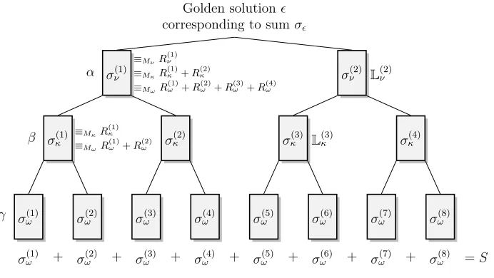
level is controlled by a new parameter β. In the last level, we finally decompose into a total of eight different subknapsacks. At this level, we use a parameter γ to denote the proportion of extra -1s in the subknapsacks.
σω(1) σω(2) σω(3) σ(4)ω σ(5)ω σω(6) σω(7) σ(8)ω
σω(1) + σω(2) + σω(3) + σ(4)ω + σ(5)ω + σω(6) + σω(7) + σω(8) =S
σκ(1) σ(2)κ σκ(3) σ(4)κ
σν(1) σν(2)
Golden solution
corresponding to sumσ
L(3)κ
L(2)ν
≡MνR (1)
ν
≡MκR (1)
κ +R
(2)
κ
≡MωR (1)
ω +R
(2)
ω +R
(3)
ω +R
(4)
ω
≡MκR (1)
κ
≡MωR (1)
ω +R
(2)
ω
γ β
α
Fig. 2.Iterative decomposition in three steps.σ(χj): partial sum,Rχ(j): target value,Mχ: modulus,α, βandγ:
proportion of additional−1s
Notation. We use a different Greek letter (, κ, ω or ν) to denote the coefficient vectors of each subknapsack. In the original knapsack, we carry on using the letter. At the first level of decomposition, we now useν(1) andν(2) for the coefficient vectors of the two subknapsacks. At
the middle level, we choose the notationκ(1)toκ(4). At the bottom level, we use the lettersω(1)
toω(8). We then let Nχ(x) denote the number of occurrences ofx∈ {−1,0,1}in the coefficient
vectorχ. For a knapsack of nelements, we have:
N(1) =n/2, N(−1) = 0, Nν(1)≈(1/4 +α)n, Nν(−1)≈αn,
Nκ(1)≈(1/8 +α/2 +β)n, Nκ(−1)≈(α/2 +β)n,
Nω(1)≈(1/16 +α/4 +β/2 +γ)n, Nω(−1)≈(α/4 +β/2 +γ)n .
We always have Nχ(0) = n−Nχ(1)−Nχ(−1). Since all these numbers need to be rounded
to integers for a concrete knapsack instance, we write ≈ instead of = above. For each of the coefficient vectorsχ(j) we introduce the corresponding partial sum:
σ(j)χ =
n
X
i=1
χ(j)i ai .
corresponding to the bottom level by Mω, we introduce 7 random values R(j)ω (for 1≤j ≤ 7)
and letR(8)ω =S−P7j=1R (j)
ω . We solve the eight modular subknapsacks:
σ(j)ω ≡R(j)ω (modMω) for 1≤j ≤8 .
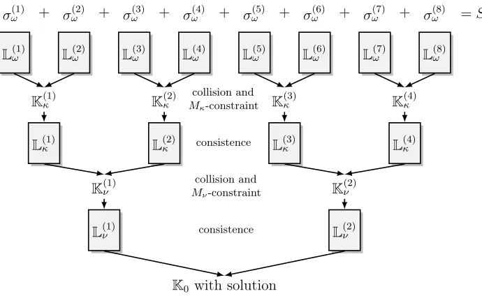
We denote by L(j)ω , the list of solutions of each of these subknapsacks. Figure 2 illustrates the
decomposition and Fig. 3 shows the merge of the lists until the golden solution is found in the last listK0.
Basic Principle and Modular Constraints. To build solutions at the middle level κ, we consider sums of two partial solutions from two neighboring lists L(2jω −1) and L(2j)ω containing
solutions of the last level. By construction, we see that:
σ(j)κ =σ(2jω −1)+σ(2j)ω ≡Rω(2j−1)+R(2j)ω (modMω)
which means that all these partial sums already have some fixed value modulo Mω. To prune
the size of the lists of solutions at this level, we add an extra constraint modulo Mκ (chosen
coprime to Mω). Thus, we introduce three random valuesR(j)κ (for 1 ≤j ≤3) and let R(4)κ = S−P3
j=1R (j)
κ . The new lists of solutions are denoted byL(j)κ .
For the first level, we proceed similarly, adding partial solutions from L(2jκ −1) and L(2j)κ .
Clearly, the resulting sums already have fixed values moduloMκ and Mω. Again, we introduce
a modulus Mν, a random value R(1)ν and we let R(2)ν =S−R(1)ν to reduce the size of the lists.
Finally, the (presumably unique) solution of the original knapsack is found by searching for a collision of the form σν(1)+σν(2) =S withσν(1) ∈L(1)ν and σ(2)ν ∈L(2)ν . Figure 2 illustrates the
technique.
To transform this informal description into a formal algorithm and to analyze its complexity, we need to specify how the lists L(j)ω are constructed. We also explain how to merge solutions
from one level to solutions at the next level and specify the choices of the moduli Mω,Mκ and Mν in the next paragraph.
Algorithmic Details. The eight lists L(j)ω can be constructed using a straightforward
adap-tation of the simple birthday paradox algorithm. It suffices to split the n elements into two random subsets of size n/2 and to assume that the 1s and -1s are evenly4 distributed between the two halves. As with the case of binary coefficient vectors, the probability of this event is the inverse of a polynomial in n. Thus by repeating polynomially many times, we recover all of L(j)ω with overwhelming probability. Assuming that the elements in L(j)ω are random modulo Mω, the expected size ofL(j)ω is:
Lω = Lω Mω
=
n
Nω(1),Nω(−1),Nω(0)
Mω
,
where Lω is the multinomial coefficient that counts the number of ways to choose Nω(1) 1s, Nω(−1) -1s and Nω(0) 0s among nelements. Since the number of ways to choose Nω(1)/2 1s,
4
L(1)ω L(2)ω L(3)ω L(4)ω L(5)ω L(6)ω L(7)ω L(8)ω
σω(1) + σ(2)ω + σω(3) + σω(4) + σω(5) + σ(6)ω + σω(7) + σω(8) =S
L(1)κ L(2)κ L(3)κ L(4)κ
L(1)ν L(2)ν
K0with solution
K(1)κ K(2)κ K(3)κ K(4)κ
K(1)ν K(2)ν
collision and
Mκ-constraint
consistence
collision and
Mν-constraint
consistence
Fig. 3.Merge of the partial solutions via check of collision and consistency
Nω(−1)/2 -1s and Nω(0)/2 0s among n/2 elements is ≈ L1/2ω for large n, the running time of
the construction of eachL(j)ω is max(|L(j)ω |,L1/2ω ).
At the middle level, the expected size ofL(j)κ is upper bounded by
Lκ = Lκ Mω·Mκ
=
n
Nκ(1),Nκ(−1),Nκ(0)
Mω·Mκ
.
This is only an upper bound on the expected size since the definition of Lκ ignores the fact
that we discard solutions that cannot be decomposed with the modular constraints of the lower level.
To construct these lists, we match values from L(2jω −1) and L(2j)ω modulo Mκ using
Al-gorithm 1 from Sect. 3.2. We let K(j)κ denote the resulting list; see Fig. 3. We then remove
inconsistent solutions fromK(j)κ in order to produceL(j)κ . We say that a solution is inconsistent
when the vector ω(2j−1)+ω(2j) contains 2s or -2s and/or does not have the number of 1s, -1s and 0s specified by Nκ(1), Nκ(−1) and Nκ(0). According to Sect. 3.2, the cost of this step is
max(|L(2jω −1)|,|L(2j)ω |,|K(j)κ |).
Proceeding in the same way, we give an upper bound on the expected size of L(j)ν by
Lν =
Lν Mω·Mκ·Mν
=
n
Nν(1),Nν(−1),Nν(0)
Mω·Mκ·Mν .
Using the same notation as above, the cost to construct the two listsL(j)ν is max(|L(2jκ −1)|,|L(2j)κ |,|K(j)ν |).
Finally, the last step is to apply the integer variant of Algorithm 1 to the two integer lists
L(1)ν and L(2)ν , obtaining a list K0 of (possibly inconsistent) solutions. The cost of this step is
To estimate the size of K0, we count the number of expected solutions in a modular merge
modulo the multiple ofMω·Mκ·Mν closest to 2n. This overestimates the size ofK0 since it is
slightly easier to find a knapsack solution modulo this value than a knapsack solution over the integers. This yields an estimate equal to:
L2ν·Mν·Mκ·Mω
2n .
If K0 contains at least one consistent solution, we obtain a solution of the initial knapsack
problem.
To conclude the description of the algorithm, we need to specify the values of the moduli
Mω, Mκ and Mν. The key idea at this point is to choose each modulus to ensure that each
solution appearing at a given level is represented (on average) by a single decomposition at the previous level. Indeed, if we add a larger modular constraint, we lose solutions from one level to the next and if we choose a smaller constraints, we construct each solution many times which increases the overall cost. Using binomials and multinomials to compute the number of decompositions we obtain the following conditions for the values of the moduli:
Mω ≈ NNκ(1)
κ(1)/2
· Nκ(−1)
Nκ(−1)/2
· Nκ(0)
Nω(1)−Nκ(1)/2,Nω(−1)−Nκ(−1)/2, ?
≈
2(1/8+α+2β−2γlog2γ−(7/8−α−2β−2γ) log2(7/8−α−2β−2γ)+(7/8−α−2β) log2(7/8−α−2β) ,
Mκ·Mω ≈ NNνν(1)/2(1)
· Nν(−1)
Nν(−1)/2
· Nν(0)
Nκ(1)−Nν(1)/2,Nκ(−1)−Nν(−1)/2, ?
≈
2(1/4+2α−2βlog2β−(3/4−2α−2β) log2(3/4−2α−2β)+(3/4−2α) log2(3/4−2α))n ,
Mν·Mκ·Mω ≈ n/2n/4
· N n/2
ν(−1),Nν(−1), ?
≈2(1/2−2αlog2α−(1/2−2α) log2(1/2−2α)+(1/2) log2(1/2))n
≈2(−2αlog2α−(1/2−2α) log2(1/2−2α))n .
The ? symbol in the above multinomials denotes the number of remaining elements (corre-sponding to 0s) after specifying the number of 1s and -1s introduced to decompose the set of 0s from the lower level.
The overall running time of the algorithm is the maximum of the individual costs to run Algorithm 1 and the construction of the eight lists, which gives:
˜
O(max(max
j |L (j)
ω |,maxj L1/2ω ,maxj |K(j)κ |,maxj |L(j)κ |,maxj |K(j)ν |,maxj |L(j)ν |,|K0|)) .
Assuming that each list has a size close to its expected value (see Sect. 3.5), the expected running time is:
T(α, β, γ) = ˜O(max(Lω,L1/2ω , L2ω Mκ
, Lκ, L2κ Mν
, Lν, L2ν·
Mν ·Mκ·Mω
2n )) .
Since none of the Kχ lists need to be stored, the amount of memory required is:
˜
Finally, there is an additional, very important, parameter to consider, the probability of success
psucc taken over the possible random choices of theR(j)χ values. This parameter is quite tricky
to estimate because it varies depending on the initial knapsack that we are solving. As an illustration, consider the knapsack whose elements are all equal to 0. It is clear that unless all the randomR(j)χ are chosen equal to 0 then the algorithm cannot succeed. As a consequence, in
this case the probability of success is very low. There are many other bad knapsacks; however, for a random knapsack, the expected probability of success is not too small (see Sect. 3.4 for a discussion).
Numerical Results for the Complexity Analysis. Minimizing the expected running time
T(α, β, γ) results in:
α= 0.0267, β= 0.0168, γ= 0.0029 .
With these values, we obtain:
Lω ≈20.532n, Lω ≈20.291n, Lκ ≈ 20.279n, Lν ≈20.217n and Mω≈20.241n, Mκ≈20.291n, Mν ≈20.267n .
As a consequence, we find that both the time and memory complexity are equal to ˜O(20.291n). We can also check that the product of the three moduli Mω·Mκ·Mν is smaller than the size
of the numbers in the initial knapsack, i.e. 2n.
However, we remark that γ is so small that for any achievable knapsack sizen, the number of−1s added at the last level is 0 in practice. Thus, in order to improve the practical choices of the number of −1s at the higher levels, it is better to adjust the minimization with the added constraint γ = 0. This leads to the alternative values:
α= 0.0194, β = 0.0119, γ = 0 .
With these values, we obtain:
Lω ≈20.463n, L
ω ≈20.295n, Lκ ≈ 20.284n, Lν ≈20.234n and Mω≈20.168n, Mκ≈20.295n, Mν ≈20.272n .
We can also remark that by choosing α = β = γ = 0, we recover the time complexity ˜
O(20.337n) given by May and Meurer [9] for the algorithm of [5]. However, in our case, the memory complexity is also ˜O(20.337n), which indicates that our algorithm can probably be improved in this respect.
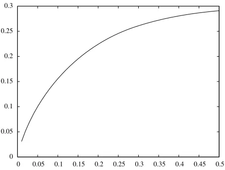
Complexity for the Unbalanced Case. We also analyzed the complexity forτ−unbalanced knapsacks. Figure 4 shows that the complexity is decreases for knapsack weight τ dropping below 0.5. Forτ larger than 0.5, the complexity increases. In this case, it is best to switch to the complementary knapsack.
0 0.05 0.1 0.15 0.2 0.25 0.3
0 0.05 0.1 0.15 0.2 0.25 0.3 0.35 0.4 0.45 0.5
Fig. 4.Exponent in the complexity for unbalanced knapsacks
four levels could not beat the three-level algorithm. Moreover, we can also consider decomposi-tions that use more values besides {−1,0,1}. In general, we could allow coefficient vectors for the subknapsacks in ranges of the form [−B, B] or [−B, B+ 1] for a (small) integer B. De-vising and analyzing the exact algorithms with these extensions, however becomes much more complex.
3.4 Analysis of the Probability of Success
In order to analyze the probability of success, it is convenient to bear in mind Fig. 2. We are starting from an unknown but fixed golden solution of the knapsack and we wish to decompose it seven times. (At each step we represent the 0s, 1s and−1s of the current coefficient vector by a tuple (i, j) wherei, j∈ {0,1,−1}.) For each of the seven splits, we add a modular constraint modulo a number very close to the total number of decompositions. For example, during the top level split, we are specifying that the sum of the left hand-side after the splitting should be congruent to R(1)ν modulo Mν, to R(1)κ +R(2)κ modulo Mκ and to R(1)ω +R(2)ω +R(3)ω +R(4)ω
moduloMω. Since the three moduli are coprime, this is equivalent to simply specifying a value
moduloMν·Mκ·Mω. Each of the decompositions is considered successful if the current golden
solution admits at least one way of splitting which satisfies the modular constraint. In this case, we focus on one of the admissible solutions for which we search for a decomposition in the level below. Fixing the solution on the left-hand side also determines the solution of the right-hand side.
Clearly, if each of the seven decompositions succeeds, the initial solution can be found by the algorithm. Assuming independence, the overall probability of success is at least equal5 to the product of the probability of success of the individual decompositions. If we do not assume independence, we can still say that the overall probability of failure is smaller than the individual probabilities of failure.
5
0 200000 400000 600000 800000 1e+06
0 200 400 600 800 1000 1200 1400 1600 1800 Knapsack Sums
Random Values
Fig. 5.Cumulative number of knapsacks (in a million) with less than a given number of not obtained values
Purely Random Heuristic Model. One approach to the analysis of the probability of an individual decomposition succeeding is to assume that for each of the possible decompositions, the resulting modular sum is a random value. We already know that there are knapsacks for which this assumption does not hold, as illustrated by the all-zero example. This is true for a large number of random, however, and is a very useful benchmark for the following analysis. For simplicity, we assume here that the number of possible decompositions is equal to the modulus
M for a large set of random knapsacks.
In this case, it is well-known that for large values of M, the proportion of modular values which are not attained after picking M random values is close toe−1'0.36.
Experimental Behavior of Decompositions. In Section 5.1, we describe an implementation of our algorithm on a 80-bit knapsack. To better understand the behavior of this implementa-tion, it is useful to determine the probability of success of each decomposition. Three levels of decomposition occur. At the top level, a balanced golden solution with 40 zeros and 40 ones needs to be split into two partial solutions with 22 ones and two -1s each. At the middle level, a golden solution with 22 ones and two -1s is to be split into two partial solutions with 12 ones and two -1s. Finally, at the bottom level, we split 12 ones and two -1s into twice 6 ones and one -1.
At the top level, the number of possible decompositions of a golden solution is larger than
40 22
40
2,2,36
number of tests to perform a statistical analysis of the modular values is very cumbersome. At the bottom level, the number of decompositions of a golden solution is 126 2
1
= 1848. This is small enough to perform significant statistics and, in particular, to study the fraction of modular values which are not obtained (depending on a random choice of 14 knapsack elements, 12 1s and two−1s, to be split). The value of the modulus used in this experiment is 1847, the closest prime to 1848.
During our experimental study, we created one million modular subknapsacks from 14 ran-domly selected values modulo 1847. Among these values 12 elements correspond to additions and 2 to subtractions. From this set we computed ( in Z1847) all of the 1848 values that can
be obtained by summing 6 out of the 12 addition elements and subtracting one of the subtrac-tion elements. In each experiment, we counted the number of values which were not obtained; the results are presented in Fig. 5. On the vertical axis we display the cumulative number of knapsacks which result in x or less unobtained values. To allow comparison with the purely random model, we display the same curve computed for one million of experiments where 1848 random numbers modulo 1847 are chosen. In particular, we see on this graph that for 99.99% of the random knapsacks we have constructed the fraction of unobtained value stays below 2/3. This means that experimentally, the probability of success of a decomposition at the bottom level is, at least, 1/3 for a very large fraction of knapsacks. Assuming independence between the probability of success of the seven splits and a similar behavior of three levels6, we conclude that for 99.93% of random knapsacks an average number of 37 = 2187 repetitions suffices to solve the initial problem.
Distribution of Modular Sums. When considering the decomposition of a given golden solution (at any level), we can construct the set Bof all left-hand sides which can appear. For this setBwe wish to study the distribution of the scalar producta·x=Pn
i=1aixi (modM), for
given knapsack weightsai. LetPa1,..,an(B, c) denote the probability that a knapsack of elements
a= (a1, .., an)∈ZnM results in the valuecmoduloM for a uniformly at random chosen solution
(x1, .., xn) from B,
Pa1,···,an(B, c) =
1
|B|
(
(x1,· · ·, xn)∈ B such that n
X
i=1
aixi ≡c (mod M)
)
.
Our main tool to theoretically study the distribution of the scalar products is the following theorem [11, Theorem 3.2]:
Theorem 1. For any setB ⊂Zn
M, the identity:
1
Mn
X
(a1,···,an)∈ZnM X
c∈ZM
Pa1,···,an(B, c)−
1
M
2
= M−1
M|B|
holds.
6
With this equation we can prove a weak but sufficient result about the proportion of missed values during a decomposition. Let Λ > 0 be an arbitrary integer. We want to find an upper bound for the fractionfΛ of “bad” knapsacks modulo M with less than M/Λ obtained values.
First, we remark that for a knapsack (a1,· · · , an) that reaches less than M/Λ values, at least
(Λ−1)M/Λ values moduloM are obtained 0 times. Since
X
c∈ZM
Pa1,···,an(B, c) = 1
some values cneed to be obtained many times. As a consequence, we find that
X
c∈ZM
Pa1,···,an(B, c)−
1
M
2
≥ Λ−1
Λ ·M·
1
M2 +
1
Λ·M·
(Λ−1)2
M2 =
Λ−1
M .
This implies that the number Nbad of “bad” knapsacks satisfies:
Nbad≤Mn· M−1
(Λ−1)|B| .
With this bound, it is possible to construct a variation of our algorithm with a provable probability of success. Given Λ ≥ 10 as a function of n, we repeat each split for 2Λ random and independently picked values. The probability of failure of such a repeated split is at most
e−2 ≈0.135, except for a “bad” knapsack. Thus, the global probability of failure on the seven
splits is smaller than 95%. By choosingM smaller than|B|(but close to it), we ensure that the total fraction of bad knapsacks is at most:
7
Λ−1 .
This fraction becomes arbitrarily small by choosing a large enough value of Λ. Note that the running time is multiplied by (2Λ)3, since there are three nested levels of decompositions. If a probability of success of 5% is not sufficient, it is possible to increase the probability by repeating the complete algorithm with independent random numbers. A polynomial number of repetition leads to a probability of success exponentially close to 1 (with the exception of the “bad” knapsacks).
3.5 Analysis of the Size of the Lists
Concerning the size of the lists that occur during the algorithm, both the simple heuristic model and the experimental results (see Section 5.1) predict that the size of the lists are always very close to the theoretical values at the bottom level and smaller (due to the overestimation) at the levels above. It remains to use Theorem 1 to give an upper bound on the size of the various lists.
For the sizes of the lists Lχ, we can use a direct application of the theorem. The set of
concern, B, is the set of all repartitions of 1s, 0s and -1s fulfilling the conditions of Lχ. The
Once again, we fix an integer Λ and consider the number FΛ of knapsacks for which more
thanM/(2Λ) valuesc have a probability that satisfies:
Pa1,···,an(B, c)≥Λ/M .
Due to Theorem 1, we find:
FΛ Mn·
M
2Λ ·
(Λ−1)2
M2 ≤
M−1
M|B| ≤
1
|B| .
As a consequence:
FΛ≤
2Λ
(Λ−1)2 · M |B|·M
n≤ 2Λ
(Λ−1)2 ·M n .
The key point is that for a knapsack which is not one of the FΛ knapsacks above and for most
values ofc(all but at mostM/(2Λ)), the size ofLχ is smaller thanΛtimes the expected value |B|/M, that is,
|Lχ| ≤ Λ|B|
M .
To bound the size of the listsKχ, we proceed slightly differently. The setBconsists of 1s, 0s
and -1s that are allowed in theLlists and are matched to constructKχ. We writeM =M1·M2,
whereM1 is the product of the active moduli for theLlist andM2 is the modulus that is added
when constructing Kχ. Let σ (modM) denote the target sum as a new modulo constraint for
elements inKχ. LetσL (modM1) andσR (modM1) respectively denote the values of the sums
in the left-side and right-side listsL. Of course, we haveσL+σR≡σ (modM1). We can write:
|Kχ|=
X
c∈ZM c≡σL (modM1)
(|B| ·Pa1,···,an(B, c))·(|B| ·Pa1,···,an(B, σ−c))
≤ X
c∈ZM c≡σL
(|B| ·Pa1,···,an(B, c))
2× X
c∈ZM c≡σR
(|B| ·Pa1,···,an(B, c))
2 1/2 . (4)
Thus to estimate the size of the listsKχ, we need to find an upper bound for the value of sums
of the form:
X
c∈ZM c≡c1 (modM1)
Pa1,···,an(B, c)
2 .
To do this, it is useful to rewrite the relation from Theorem 1 as:
1
Mn
X
(a1,···,an)∈ZnM X
c∈ZM
Pa1,···,an(B, c)
2= M +|B| −1
Given Λ, we let GΛ denote the number of knapsacks for which more than M1/(8Λ) values c1
have a sum of squared probabilities that satisfy:
X
c∈ZM c≡c1 (modM1)
Pa1,···,an(B, c)
2 ≥ Λ2 M12M2
.
We find that
GΛ Mn ·
M1
8Λ · Λ2 M12M2
≤ M+|B| −1
M|B| ;
and as a consequence
GΛ≤
8
Λ ·
M +|B| |B| ·M
n .
Moreover, we can check with our concrete algorithm that we always have |B| ≥ M for the construction of the lists Kχ. Thus we have GΛ ≤(16/Λ)Mn.For a knapsack which is not one
of the GΛknapsacks above and for most values 7 ofσLmodM1, the size of Kχ is smaller than Λ2 times the expected value|B|2/(M2
1 M2), that is,
|Kχ| ≤
Λ2|B|2 M2
1 ·M2 .
Note, that this bound includes the case |K0|.
3.6 Provable Variant of the Concrete Algorithm
Following the ideas presented in Sect. 3.4, we can now describe a variant of our concrete al-gorithm with provable probabilistic run-time and space requirements. First, fix a large enough value ofΛ. We redefine the notion of a “bad” knapsack in this section, by saying that a knapsack is bad if it fails to fulfill one of the three criteria developed in Sect. 3.4 and Sect. 3.5. That is, if there are too many values that yield incorrect splits or lists of typeLorKwhich are too large. We find that the total fraction of bad knapsacks is smaller than
7
1
Λ−1 + 2Λ
(Λ−1)2 +
16
Λ
≤ 140
Λ forΛ≥7 .
By choosing a large enough value for Λ, this fraction can become arbitrarily small.
Once again, we consider a variation of the concrete algorithm where at each level we repeat the choice of random numbers often enough to be successful. For a “good” knapsack there are three ways a decomposition can fail (or a merge can fail, depending on whether we are adopting the view of Fig. 3 or of Figure 2). Firstly, we could choose a random value which does not permit a decomposition of the golden solution; Secondly, we could choose a random value which makes Lχ overflow; Thirdly, we could choose a random value which makesKχ overflow. Note that the
last two events can be detected, in which case we erase the lists that have been constructed for
7For all but at most 2M
this random value and turn to the next. For each modulus, the proportion of random values which are incorrect with respect to at least one criteria is smaller than
Λ−1
Λ +
1 2Λ +
2
8Λ = 1−
1 4Λ .
Thus by repeating each split 8Λ times, we make sure that the probability of failure of a given split is at moste−2. Once again, this yields a global probability of success of 5%, which becomes exponentially close to 1 by repeating polynomially many times. Given a real ε >0, by setting
Λ= 2ε n we obtain the following theorem:
Theorem 2. For any real ε > 0 and for a fraction of at least 1−140·2−ε n of equibalanced knapsacks with density D < 1 given by an n-tuple (a1,· · · , an) and a target value S, if =
(1,· · · , n) is a solution of the knapsack then the algorithm described in Sect. 3.3 modified as
above finds the solution sought after in time O˜(2(0.291+3ε)n).
We recall that in the theorem, the termequibalancedmeans that the solutioncontains exactly the same number of 0s and 1s.
4 Memory Complexity Improvement
In this section we first show a new algorithm of constant memory requirement and running time ˜O(23n/4). We then show how to decrease its time complexity down to ˜O(20.72n) using a
technique similar to Howgrave-Graham and Joux [5]. Finally, we show a time memory tradeoff for Schroeppel-Shamir’s algorithm down to ˜O(2n/16) memory.
4.1 An Algorithm with Running Time ˜O(23n/4) and Memory ˜O(1)
We describe a simple algorithm that solves the knapsack problem in time ˜O(23n/4) and constant memory, using a meet-in-the-middle attack. This is done by formulating the meet-in-the-middle attack as a collision search problem (see [15]); then a constant memory cycle-finding algorithm can be used.
We define two functions f1, f2:{0,1}n/2→ {0,1}n/2:
f1(x) = n/2
X
i=1
aixi mod 2n/2, f2(y) =S− n
X
i=n/2+1
aiyi mod 2n/2
wherexi denotes thei-th bit ofx, and similarly foryi. If we can find x, y∈ {0,1}n/2 such that f1(x) =f2(y), then we get:
n/2
X
i=1 aixi+
n
X
i=n/2+1
aiyi =S mod 2n/2 .
probability roughly 2−n/2. Below we show that we can generate such random solution in time ˜
O(2n/4) and constant memory. This gives an algorithm with total running time ˜O(23n/4) and
constant memory.
From the two functions f1,f2 we define the functionf :{0,1}n/2→ {0,1}n/2 where:
f(x) =
(
f1(x) ifg(x) = 0
f2(x) ifg(x) = 1
whereg:{0,1}n/2 → {0,1}is a random bit function. Then a collisionf(x) =f(y) forf gives a
desired collision f1(x) =f2(y) with probability 1/2. The functionf :{0,1}n/2→ {0,1}n/2 is a
random function, therefore using Floyd’s cycle finding algorithm [6] we can find a collision for
f in time 2n/4 and constant memory.
However we need to obtain a random collision whereas Floyd’s cycle finding algorithm is likely to produce always the same collision. A simple solution is to further randomize the functionf; more precisely we apply Floyd’ cycle-finding algorithm to f0 :{0,1}n/2 → {0,1}n/2
withf0(x) =P(f(x)), where P is a random permutation in{0,1}n/2. Then a new permutation P is used every time a new collision (x, y) is required for f.
4.2 An Algorithm with Running Time ˜O(20.72n) and Memory ˜O(1)
In this section we show how to slightly decrease the running time down to ˜O(20.72n), still with constant memory; for this we use the Howgrave-Graham–Joux technique recalled in Sect. 2.1. Again for simplicity we assume thatn is a multiple of 4, and that the Hamming weight of the knapsack solutionis exactlyn/2. As in (3) we writeS as the sumσ1+σ2 of two subknapsacks
with Hamming weightn/4 chosen among the nknapsack elements,
n
X
i=1 aiyi
| {z }
σ1 +
n
X
i=1 aizi
| {z }
σ2
=S .
We letW be the set ofn-bit strings of Hamming weightn/4. We have #W = 2h(1/4) '20.81n. We define the two functionsf1, f2 :W → {0,1}h(1/4)n:
f1(y) = n
X
i=1
aiyi mod 2h(1/4)n, f2(z) =S− n
X
i=1
aizi mod 2h(1/4)n
whereyi denotes thei-th bit ofy, and similarly for zi. We consider y, z ∈W such that:
f1(y) =f2(z) (5)
equivalently:
n
X
i=1 aiyi+
n
X
i=1
Since f1 and f2 are random functions heuristically there are 2h(1/4)nsolutions to (5).
More-over given the correct solution of the knapsack, as in Sect. 2.1 there are n/2n/4
'2n/2 ways of
writing this correct solution as
n
X
i=1 aiyi+
n
X
i=1
aizi=S
where y and z both have Hamming weight n/4. All these 2n/2 solutions are solutions of (5). Therefore the probabilitypthat a random solution of (5) leads to the correct knapsack solution is:
p= 2
n/2
2h(1/4)n '2 −.31n .
The input space of f1,f2 has size 2h(1/4)n. Therefore using the same cycle-finding algorithm
as in the previous section, a random solution of (5) can be found in time ˜O(2h(1/4)n/2). The total time complexity is therefore:
˜
O(2h(1/4)n/2)/p= ˜O(2h(1/4)n/2)·2(h(1/4)−1/2)n
= ˜O(2(3h(1/4)/2−1/2)n) = ˜O(2.72n) .
Finally, we note that it is possible to further improve this complexity by adding −1s in the decomposition (as in Sect. 3) but the time complexity improvement is almost negligible.
4.3 A Time-Memory Tradeoff on Schroeppel-Shamir down to 2n/16 Memory
The original Schroeppel-Shamir algorithm works in time ˜O(2n/2) and memory ˜O(2n/4). In this section we describe a continuous time-memory tradeoff down to ˜O(2n/16) memory. That is we describe a variant of Schroeppel-Shamir with:
Running time: ˜O(2(11/16−ε)n), Memory: ˜O(2(1/16+ε)n)
for any 0 ≤ ≤ 3/16. For simplicity we first describe the algorithm with exactly ˜O(2n/16)
memory. We write the knapsack asS =σ1+σ2+σ3+σ4 as in (2) where eachσi is a knapsack
of n/4 elements , that is:
σ1 = n/4
X
i=1
iai, σ2 = n/2
X
i=n/4+1
iai, σ3= 3n/4
X
i=n/2+1
iai, σ4 = n
X
i=3n/4+1 iai .
We guess three valuesR1,R2 andR3 of 3n/16-bit each and we letR4 such thatR1+R2+ R3+R4 =S mod 23n/16. We consider the four subknapsack equations
σi=Ri mod 23n/16 .
We solve these four equations independently by using the original Schroeppel-Shamir algo-rithm. Therefore in time ˜O(2n/8) and memory ˜O(2n/16) we obtain four lists {σ1}, {σ2}, {σ3}
these four lists using the same merging procedure as in the original Schroeppel-Shamir algo-rithm; since each list has size ˜O(2n/16), the merging procedure runs in time ˜O(2n/8) and memory
˜
O(2n/16). Since we have guessed three values of 3n/16-bit each, the total running time is:
˜
O(23n/16)3·O˜(2n/8) + ˜O(2n/8)= ˜O(211n/16)
as required, and the memory consumption is ˜O(2n/16).
It is easy to generalize the previous algorithm to memory ˜O(2(1/16+ε)n) for any 0≤ <3/16. For this we take theRi’s of size (3/16−ε)n-bit each. We can still build the four lists{σi}in time
˜
O(2n/8) using Schroeppel-Shamir, but this time the size of the lists is ˜O(2(1/16+ε)n), therefore it requires ˜O(2(1/16+ε)n) memory. The merging procedure now runs in time ˜O(2(1/8+2ε)n), still with memory ˜O(2(1/16+ε)n). Therefore the total running time is:
˜
O(2(3/16−ε)n)3·O˜(2n/8) + ˜O(2(1/8+2ε)n)= ˜O(2(11/16−ε)n)
as required, for a memory consumption ˜O(2(1/16+ε)n).
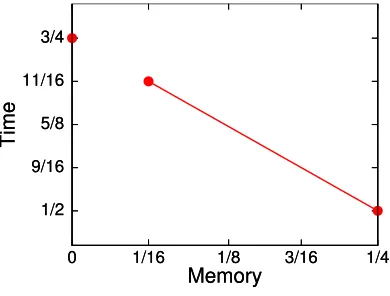
1/2 9/16 5/8 11/16 3/4
0 1/16 1/8 3/16 1/4
Time
Memory
1/2 9/16 5/8 11/16 3/4
0 1/16 1/8 3/16 1/4
Time
Memory
Fig. 6.Illustration of the existing gap between our constant memory algorithm and our time-memory tradeoff for Schroeppel-Shamir
Surprisingly there remains a gap between our variant of Schroeppel-Shamir with ˜O(2n/16) memory and our constant memory algorithm from Sect. 4.1; see Fig. 6 for an illustration. Namely we were unable to find a variant of Schroeppel-Shamir requiring less than ˜O(2n/16) memory, nor a cycle-based algorithm requiring more than ˜O(1) memory.
5 Implementation and Experimental Evidence
5.1 Implementation of the Improved Time Complexity Algorithm
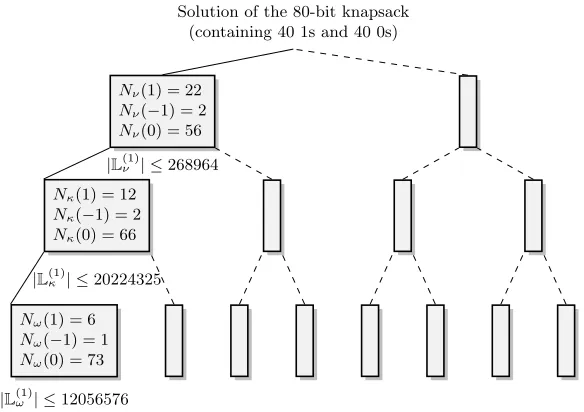
knapsacks, we ran our implementation several times, choosing new random modular constraints for each execution, until a solution was found. As shown in Fig. 7, we added two -1s at the first level, one -1 at the second and none at the third level. At the same time, we collected some statistics about the behavior of our code.
The total running time to solve the 50 knapsacks was 14 hours and 50 minutes on a IntelR
CoreTMi7 CPU M 620 at 2.67GHz. The total number of repetitions of the basic algorithm was equal to 280. We observed that a maximum of 16 repetitions (choice of a different random value in level ν) was sufficient to find the solution. Also, 53% of the 50 random knapsacks needed only up to 4 repetitions. On average, each knapsack required 5.6 repetitions. More precisely, the distribution of the number of repetitions is presented in Table 1.
Table 1.Number of repetitions for 50 random knapsacks until a solution was found.
Number of Number of Number of Number of repetitions corresponding knapsacks repetitions corresponding knapsacks
1 8 2 6
3 9 4 4
5 2 6 5
7 1 8 1
9 1 10 5
11 4 12 1
13 0 14 1
15 0 16 2
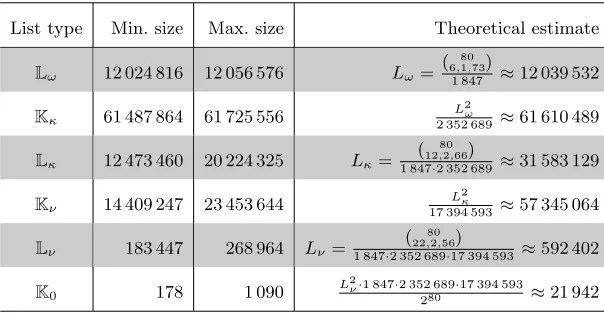
Table 2.Experimental versus theoretical sizes of the intermediate lists.
List type Min. size Max. size Theoretical estimate
Lω 12 024 816 12 056 576 Lω=
( 80 6,1,73)
1 847 ≈12 039 532
Kκ 61 487 864 61 725 556
L2 ω
2 352 689≈61 610 489
Lκ 12 473 460 20 224 325 Lκ=
( 80 12,2,66)
1 847·2 352 689≈31 583 129
Kν 14 409 247 23 453 644
L2κ
17 394 593≈57 345 064
Lν 183 447 268 964 Lν=
( 80 22,2,56)
1 847·2 352 689·17 394 593 ≈592 402
K0 178 1 090
L2ν·1 847·2 352 689·17 394 593
280 ≈21 942
Table 2 that the sizes ofLω andKκ are very close to the predicted values and do not vary a lot.
We already mentioned in Sect.3.3, that the prediction Lκ and Lν ignores the loss of solutions
which are incompatible with the modular constraints of the lower levels. The actual sizes of the lists is therefore smaller than the predicted one. The effect is forwarded from level κ to levelν
resulting in an even bigger gap between theory and practice for|Lν|and|Kν|. The experimental
size of K0 counts inconsistent solutions corresponding to collisions over the integers. We recall
that our theoretical estimate upper bounds the size as it counts collisions moduloMω·Mκ·Mν,
a number close to 280.
Nω(1) = 6
Nω(−1) = 1
Nω(0) = 73
Nκ(1) = 12
Nκ(−1) = 2
Nκ(0) = 66
Nν(1) = 22
Nν(−1) = 2
Nν(0) = 56
Solution of the 80-bit knapsack (containing 40 1s and 40 0s)
|L(1)ν | ≤268964
|L(1)κ | ≤20224325
|L(1)ω | ≤12056576
Fig. 7.Decomposition of a single solutionσ for an equibalanced knapsack of size 80. The decomposition into
Nχ(1) 1s,Nχ(−1) -1sandNχ(0) 0sis the same within each levelχ∈ {ν, κ, ω}
Some More Tests. We also performed additional tests on 240 random knapsacks where we repeated the search for a solution 10 times per knapsack. Figure 8 shows the distribution of necessary repetitions until the solution was found. We observe an average of µ = 5.47 and a maximum of 41 repetitions. In 95% of the cases less than 16 repetitions were enough to find the solution. Furthermore, the results seem to be conform with a random variable following the geometric distribution of expected value µ where we assume independence for each decompo-sition and level and the same probability of success 1/µ. Figure 8 also depicts the probability distribution of the random variable. None of the tested random knapsacks was distinctly easier or more difficult to solve than the others within the 10 runs.
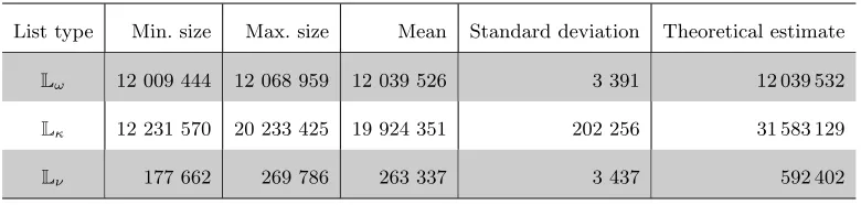
The sizes of the intermediate lists Lω,Lκ and Lν are given in Table 3. We present the
0 2 4 6 8 10 12 14 16 18
0 5 10 15 20 25 30 35 40 45
percent
repetitions
experiments 100*exp((x-1)*log(1-1/µ))
Fig. 8.Percentage of 240 random knapsacks, each run 10 times, per number of repetitions (red bar); Random variable of geometric distribution in valuesx, probabilitiespx= 100·exp((x−1)·log(1−1/µ)),whereµis the
average number of repetitions (green - -)
Table 3.Experimental sizes of the intermediate lists for 240 random knapsacks.
List type Min. size Max. size Mean Standard deviation Theoretical estimate
Lω 12 009 444 12 068 959 12 039 526 3 391 12 039 532
Lκ 12 231 570 20 233 425 19 924 351 202 256 31 583 129
Some Results with n= 96. We also tested the algorithm on equibalanced 96-bit knapsacks. However, it was not possible to add the optimal number of -1s, because some of the lists required too much memory. Instead, we used the following suboptimal choices:
– Split the initial knapsack into two subknapsack with 25 ones and one -1.
– Split again into subknapsacks with 14 ones and two -1s.
– Finally split into subknapsacks with 7 ones and one -1.
The chosen moduli are Mω = 6 863, Mκ = 248 868 793 and Mν = 42 589. We tried 5 different
knapsacks and solved all of them with an average number of repetitions equal to 7.8. The runtime for a single trial is 47 minutes on a IntelR XeonTM CPU X5560 at 2.80GHz using 13 Gbytes of memory8.
For comparison, we also ran on the same machine the latest version of our implementation of a practical variant of the Howgrave-Graham–Joux algorithm. This variant took an average of 15 minutes to solve a knapsack on 96 bits, using 1.6 Gbytes of memory. However, this program is much more optimized for the practical parameters. Moreover, it contains some wild heuristics to reuse the computations of intermediate lists many times, in order to run faster. The new algorithm can probably take practical profit of similar tricks. As a consequence, the runtimes on 96 bits are not so far from each other. We expect the cross-over point to occur aroundn= 128, which means that 96 bits is close to the cross-over point between the two algorithms.
5.2 Constant Memory Algorithm
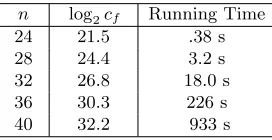
We have also implemented the constant memory algorithm based on cycle finding from Sect. 4.1. The results summarized in Table 4 seem consistent with a ˜O(23n/4) time complexity. The implementation was running on a Intel Core 2 Duo P8400 (2.26 GHz).
n log2cf Running Time
24 21.5 .38 s 28 24.4 3.2 s 32 26.8 18.0 s 36 30.3 226 s 40 32.2 933 s
Table 4.Knapsack sizen, log2 number of callscf tof and running time on a C implementation running on a
Intel Core 2 Duo P8400 (2.26 GHz), averaged over 10 executions.
6 Conclusion
We have extended the Howgrave-Graham–Joux technique to get an algorithm with running time down to ˜O(20.291n). An implementation of an accessible example of 80 knapsack elements shows the practicability of the method. We have described a constant memory algorithm based on cycle finding with running time ˜O(20.72n), and also a time-memory tradeoff for Schroeppel-Shamir.
Acknowledgments. We would like to thank Alexander May and Alexander Meurer for point-ing out the inconsistency issue in Howgrave-Graham–Joux algorithm. We also thank Dan Bern-stein for helpful comments on a preliminary version of this work.
References
1. Mikl´os Ajtai. The shortest vector problem in L2is NP-hard for randomized reductions (extended abstract). InSTOC’98, pages 10–19, 1998.
2. Anja Becker, Jean-S´ebastien Coron, and Antoine Joux. Improved generic algorithms for hard knapsacks. Eurocrypt 2011.
3. Matthijs J. Coster, Antoine Joux, Brian A. LaMacchia, Andrew M. Odlyzko, Claus-Peter Schnorr, and Jacques Stern. Improved low-density subset sum algorithms. Computational Complexity, 2:111–128, 1992. 4. M. R. Garey and David S. Johnson. Computers and Intractability: A Guide to the Theory of
NP-Completeness. W. H. Freeman, 1979.
5. Nick Howgrave-Graham and Antoine Joux. New generic algorithms for hard knapsacks. In EURO-CRYPT’2010, pages 235–256, 2010.
6. Donald E. Knuth. The Art of Computer Programming, Volume II: Seminumerical Algorithms, 2nd Edition. Addison-Wesley, 1981.
7. Jeffrey C. Lagarias and Andrew M. Odlyzko. Solving low-density subset sum problems. J. ACM, 32(1):229– 246, 1985.
8. Arjen K. Lenstra, Hendrik W. Lenstra, and L´aszl´o Lov´asz. Factoring polynomials with rational coefficients. Mathematische Annalen, 261:515–534, 1982.
9. Alexander May and Alexander Meurer. Personal communication.
10. Ralph C. Merkle and Martin E. Hellman. Hiding information and signatures in trapdoor knapsacks. IEEE Transactions On Information Theory, 24:525–530, 1978.
11. Phong Q. Nguyen, Igor E. Shparlinski, and Jacques Stern. Distribution of modular sums and the security of the server aided exponentiation. InProgress in Computer Science and Applied Logic, volume 20 ofFinal proceedings of Cryptography and Computational Number Theory workshop, Singapore (1999), pages 331–224, 2001.
12. Claus-Peter Schnorr. A hierarchy of polynomial time lattice basis reduction algorithms. Theor. Comput. Sci., 53:201–224, 1987.
13. Richard Schroeppel and Adi Shamir. A T = O(2n/2), S = O(2n/4) algorithm for certain NP-complete problems. SIAM J. Comput., 10(3):456–464, 1981.
14. Adi Shamir. A polynomial time algorithm for breaking the basic Merkle-Hellman cryptosystem. In CRYPTO’82, pages 279–288, 1982.
15. Paul C. van Oorschot and Michael J. Wiener. Improving implementable meet-in-the-middle attacks by orders of magnitude. InCRYPTO, pages 229–236, 1996.