GNUC: A New Universal Composability Framework
∗Dennis Hofheinz† Victor Shoup‡
December 11, 2012
Abstract
We put forward a framework for the modular design and analysis of multi-party protocols. Our framework is called “GNUC” (with the recursive meaning “GNUC’s Not UC”), already alluding to the similarity to Canetti’s Universal Composability (UC) framework. In particular, like UC, we offer a universal composition theorem, as well as a theorem for composing protocols with joint state.
We deviate from UC in several important aspects. Specifically, we have a rather different view than UC on the structuring of protocols, on the notion of polynomial-time protocols and attacks, and on corruptions. We will motivate our definitional choices by explaining why the definitions in the UC framework are problematic, and how we overcome these problems.
Our goal is to offer a framework that is largely compatible with UC, such that previous results formulated in UC carry over to GNUC with minimal changes. We exemplify this by giving explicit formulations for several important protocol tasks, including authenticated and secure communication, as well as commitment and secure function evaluation.
1
Introduction
Modular protocol design. The design and analysis of complex, secure multi-party protocols requires a high degree of modularity. By modularity, we mean that protocol components (i.e., subprotocols) can be analyzed separately; once all components are shown secure, the whole protocol should be.
Unfortunately, such a secure composition of components is not a given. For example, while one instance of textbook RSA encryption with exponente= 3 may be secure in a weak sense, all security is lost if three participants encrypt the same message (under different moduli), see [H˚as88]. Further-more, zero-knowledge proof systems may lose their security when executed concurrently [GK96]. In both cases, multiple instances of the same subprotocol may interact in strange and unexpected ways.
The UC framework. However, if security of each component in arbitrary contexts is proven, then, by definition, secure composition and hence modular design is possible. A suitable security notion (dubbed “UC security”) was put forward by Canetti [Can01], building on a series of earlier works [GMW86, Bea92, MR92, Can00].
Like earlier works, UC defines security through emulation; that is, a (sub)protocol is considered secure if it emulates an ideal abstraction of the respective protocol task. In this, one system Π
∗
First version: June 6, 2011; second version: Dec. 11, 2012 (improved exposition, improved modeling of static corruptions, no other definitional changes)
†
Karlsruhe Institute of Technology
‡
emulates another system F if both systems look indistinguishable in arbitrary environments, and even in face of attacks. In particular, for every attack on Π, there should be a “simulated attack” on F that achieves the same results.
Universal composition. Unlike earlier works, UC features a universal composition theorem (hence the name UC): if a protocol is secure, then even many instances of this protocol do not lose their security in arbitrary contexts. Technically, if Π emulates an ideal functionalityF, then we can replace allF-instances with Π-instances in arbitrary larger protocols that useF as a subprotocol. This UC theorem has proven to be a key ingredient to modular analysis. Since the introduction of the UC framework in 2001, UC-compatible security definitions for most conceivable cryptographic tasks have been given (see, e.g., [Can05] for an overview). This way, highly nontrivial existing (e.g., [CLOS02, GMP+08]) and new (e.g., [Bar05, BCD+09]) multi-party protocols could be explained and analyzed in a structured fashion. In fact, a security proof in the UC framework has become a standard litmus test for complex multi-party computations. For instance, by proving that a protocol emulates a suitable ideal functionality, it usually becomes clear what exactly is achieved, and against which kinds of attacks.
The current UC framework. The technical formulation of the UC framework has changed over time, both correcting smaller technical bugs, and extending functionality. As an example of a technical bug, the notion of polynomial runtime in UC has changed several times, because it was found that earlier versions were not in fact compatible with common constructions or security proofs (see [HUMQ09] for an overview). As an example of an extension, the model of computation (and in particular message scheduling and corruption aspects) in UC has considerably evolved. For instance, earlier UC versions only allowed the atomic corruption of protocol parties; the most recent public UC version [Can05] allows a very fine-grained corruption of subprotocol parts, while leaving higher-layer protocols uncorrupted.
Issues in the UC framework. In the most recent public version UC05 [Can05], the UC frame-work has evolved to a rather complex set of rules, many of which have grown historically (e.g., the control function, a means to enforce global communication rules). As we will argue below, this has led to a number of undesirable effects.
Composition theorem. As a first example, we claim that, strictly speaking, the UC theorem itself does not hold in UC05. The reason has to do with the formalization of the composition operation, i.e., the process of replacing one subprotocol with another. In UC05, the composition operation replaces the code of an executed program party-internally, without changing even the interface to the adversary. Hence, an adversary may not even know which protocol a party is running.
However, during the proof of the composition theorem, we have to change exactly those parts of the adversary that relate to the replaced subprotocol instances. Because there is no way for the adversary to tell which program a party runs, it is hence not clear how to change the adversary.
We give a more detailed description of in §11.2, along with a counterexample, which we briefly sketch here (using traditional UC terminology).
We start with a one-party protocol Π0 that works as follows. It expects an initialization message from the environment Z, which it forwards to the adversary A. After this, it awaits a bit b from
A, which it forwards to Z. We next define a protocol Π0
We hope that the reader agrees that Π0
1 emulates Π0 in the UC05 framework. Indeed, the simulator A0, which is attacking Π0, uses an internal copy of an adversaryA0
1 that is supposed to be attacking Π01. WhenA01 attempts to send a bitbto Π01,A0 instead sends the bit 1−bto Π0. We think that this is not a quirk of the UC05 framework — in fact, we believe that Π0
1 should emulate Π0 in any reasonable UC framework.
So now consider a one-party protocol Π that works as follows. Π expects an initial message from Z, specifying a bitc; ifc= 0, it initializes a subroutine running Π0, and ifc= 1, it initializes a subroutine running Π0
1. However, the machine ID assigned to the subroutine is the same in either case. When Π receives a bit from its subroutine, it forwards that bit to Z.
The composition theorem says that we should be able to substitute Π01 for Π0 in Π, obtaining a protocol Π1 that emulates Π. Note that in Π1, the subroutine called is Π01, regardless of the value ofc. However, it is impossible to build such a simulator — intuitively, the simulator would have to decide whether to invert the bit, as inA0, or not, and the simulator simply does not have enough information to do this correctly.
In any fix to this problem, the adversary essentially must be able to determine not only the program being run by a given machine, but also the entire protocol stack associated with it, in order to determine whether it belongs to the relevant subprotocol or not.
Trust hierarchy. Next, recall that UC05 allows very fine-grained corruptions. In particular, it is possible for an adversary to corrupt only a subroutine (say, for secure communication with another party) of a given party. In this, each corruption must be explicitly “greenlighted” by the protocol environment, to ensure that the set of corrupted parties does not change during composition. Specifically, this explicit authorization step prevents a trivial simulation in which the ideal adversary corrupts all ideal parties.
We claim that the UC05 corruption mechanism is problematic for two reasons. First, usually the set of (sub)machines in a real protocol and in an ideal abstraction differ. As an example, think of a protocol that implements a secure auction ideal functionality, and in the process uses a subprotocol for secure channels. The real protocol is comprised of at least two machines per party (one for the main protocol, one for the secure channels subprotocol). However, an ideal functionality usually has only one machine per party. Now consider a real adversary that corrupts only the machine that corresponds to a party’s secure channels subroutine. Should the ideal adversary be allowed to corrupt the only ideal machine for this party? How should this be handled generally? In the current formulation of UC05, this is simply unclear. (We give more details and discussion about this in§11.3.)
Second, consider the secure auctions protocol again. In this example, an adversary can imper-sonate a party by only corrupting this party’s secure channels subroutine. (All communication is then handled by the adversary in the name of the party.) Hence, for all intents and purposes, such a party should be treated as corrupted, although it formally is not. This can be pushed further: in UC05, the adversary can actually bring arbitrary machines (i.e., subroutines) into existence by sending them a message. There are no restrictions on the identity or program of such machines; only if a machine with that particular identity already exists is the message relayed to that machine. In particular, an adversary could create a machine that communicates with other parties in the name of an honest party before that party creates its own protocol stack and all its subroutines. This has the same effect as corrupting the whole party, but without actually corrupting any machine. (See§11.3 for more details.)
all necessary subprotocols of an implementation. In particular, this means that formally, the in-terface of an ideal protocol must depend on the complexity of the intended implementation. This complicates the design of larger protocols, which, e.g., must adapt their own padding requirements to those of their subprotocols. Similar padding issues arise in the definition of poly-time adversaries. This situation is somewhat unsatisfying from an aesthetic point of view, in particular since such padding has no intuitive justification. We point out further objections against the UC05 notion of polynomial runtime in§11.7.
None of the objections we raise point to gaps in security proofs of existing protocols. Rather, they seem artifacts of the concrete technical formulation of the underlying framework.
GNUC. One could try to address all those issues directly in the UC framework. However, this would likely lead to an even more complex framework; furthermore, since significant changes to the underlying communication and machine model seem necessary, extreme care must be taken that all parts of the UC specification remain consistent. For these reasons, we have chosen to develop GNUC (meaning “GNUC’s not UC”, and pronounced g-NEW-see) from scratch as an alternative to the UC framework. In GNUC, we explicitly address all of the issues raised with UC, while trying to remain as compatible as possible with UC terminology and results.
Before going into details, let us point out our key design goals:
Compatibility with UC. Since the UC issues we have pointed out have nothing to do with concrete security proofs for protocols, we would like to make it very easy to formulate existing UC results in GNUC. In particular, our terminology is very similar to the UC terminology (although the technical underpinnings differ). Also, we establish a number of important UC results (namely, the UC theorem, completeness of the dummy adversary, and composition with joint state) for GNUC. We also give some example formulations of common protocol tasks. Anyone comfortable in using UC should also feel at home with GNUC.
Protocol hierarchy. We establish a strict hierarchy of protocols. Every machine has an identity that uniquely identifies its position in the tree of possible (sub)protocols. Concretely, any machineM0 invoked by another machine M has an identity that is a direct descendant of that of
M. The program of a machine is determined by its identity, via aprogram map, which maps the machine’s identity to a program in a library of programs. Replacing a subprotocol then simply means changing the library accordingly. This makes composition very easy to formally analyze and implement. Furthermore, the protocol hierarchy allows to establish a reasonable corruption policy (see below).
Hierarchical corruptions. Motivated by the auction example above, we formulate a basic premise:
if any subroutine of a machine M is corrupt, then M itself should be viewed as corrupt.
Polynomial runtime. Our definition of polynomial runtime should avoid the technical pitfalls that led to current UC runtime definition. At the same time, it should be convenient to use, without unnatural padding conventions (except, perhaps, in extreme cases). A detailed description can be found in our technical roadmap in §2. However, at this point we would like to highlight a nice property that our runtime notion shares with that of UC05. Namely, our poly-time notion is closed under composition, in the following sense: if one instance of a protocol is poly-time, then many instances are as well. Furthermore, if we replace a poly-time subprotocol Π0 of a poly-time protocol Π with a poly-time implementation Π0
1 of Π0, then the resulting protocol is poly-time as well. (While this sounds natural, this is not generally the case for other notions of poly-time such as the one from [HUMQ09].)
Other related work. Several issues in the UC framework have been addressed before, sometimes in different protocol frameworks. In particular, the issues with the UC poly-time notion were already recognized in [HMQU05, K¨us06, HUMQ09]. These works also propose solutions (in different protocol frameworks); we comment on the technical differences in §11.7,§11.8, and§11.9. The UC issues related to corruptions have already been recognized in [CCGS10].
Besides, there are other protocol frameworks; these include Reactive Simulatability [BPW07], the IITM framework [K¨us06], and the recent Abstract Cryptography [MR11] framework. We comment on Reactive Simulatability and the IITM framework in §11.9 and §11.8. The Abstract Cryptography framework, however, focuses on abstract concepts behind cryptography and has not yet been fully specified on a concrete machine level.
2
Roadmap
In this section, we give a high-level description of each of the remaining sections.
Section 3: machine models
In this section, we present a simple, low-level model of interactive machines (IMs)and systems of IMs. Basically, a system of IMs is a network of machines, with communication based onmessage passing. Execution of such a system proceeds as a series of activations: a machine receives a message, processes it, updates its state, and sends a message to another machine.
Our model allows an unbounded number of machines. Machines are addressed by machine IDs. If a machine sends a message to a machine which does not yet exist, the latter is dynamically generated. A somewhat unique feature of our definition of a system of IMs is the mechanism by which the program of a newly created IM is determined. Basically, a system of IMs defines alibrary of programs, which is a finite map fromprogram names toprograms (i.e., code). In addition, the system defines a mapping from machine IDs to program names. Thus, for a fixed system of IMs, a machine’s ID determines its program.
Section 4: structured systems of interactive machines
a sandbox that ensures that all restrictions are met. We give here a brief outline of what these restrictions are meant to provide.
In a structured system of IMs, there are three classes of machines: environment,adversary, and protocol. There will only be one instance of an environment, and only one instance of an adversary, but there may be many instances of protocol machines, running a variety of different programs.
Protocol machines have IDs of the formhpid,sidi. Here,pid is called aparty ID (PID)andsid is called asession ID (SID). Machines with the same SID run the same program, and are considered peers. The PID serves to distinguish these peers. Unfortunately, the term “party” carries a number of connotations, which we encourage the reader to ignore completely. The only meaning that should be applied to the term “party” is that implied by the rules regarding PIDs. We will go over these rules shortly.
We classify protocol machines as eitherregular orideal. The only thing that distinguishes these two types syntactically is their PID: ideal machines have a special PID, which is distinct from the PIDs of all regular machines. Regular and real machines differ, essentially, in the communication patterns that they are allowed to follow. An ideal machine may communicate directly (with perfect secrecy and authentication) with any of its regular peers, as well as with the adversary.
A regular machine may interact with its ideal peer, and with the adversary; it may not interact directly with any of its other regular peers, although indirect interaction is possible via the ideal peer. A regular machine may also pass messages to subroutines, which are also regular machines. Subroutines of a machineM may also send messages toM, theircaller.
Two critical features of our framework are that regular machines are only created by being called, as above, and that every regular machine has a unique caller. Usually, the caller of a regular machine M will be another regular machine; however, it may also be the environment, in which case, M is a “top level” machine. The environment may only communicate directly with such top-level regular machines, as well as with the adversary.
Another feature of our framework is that the SID of a regular machine specifies the name of the program run by that machine, and moreover, the SID completely describes the sequence of subroutine calls that gave rise to that machine. More specifically, an SID is structured as a “pathname”, and when a machine with a given pathname calls a subroutine, the subroutine shares the same PID as the caller, and the subroutine’s SID is a pathname that extends the pathname of the caller by one component, and this last component specifies (among other things) the program name of the subroutine.
One final important feature of our framework is that the programs of regular machines must “declare” the names of the programs that they are allowed to call as subroutines. These declarations are strictly enforced at run time.
Execution of such a system proceeds as follows. First, the environment is activated. After this, as indicated by the restrictions described above, control may pass between
• the environment and a top-level regular machine,
• a regular machine and its ideal peer,
• a regular machine and its caller,
• a regular machine and one of its subroutines,
• the adversary and the environment, or
We close this section with the definition of thedummy adversary(usually denoted byAd). This
is a specific adversary that essentially acts as a “wire” connecting the environment to protocol machines.
Section 5: protocols
This section defines what we mean by a protocol. Basically, a protocol Π is a structured system of IMs, minus the environment and adversary. In particular, Π defines a map from program names to programs. The subroutine declarations mentioned above define a static call graph, with program names as nodes, and with edges indicating that one program may call another. The requirement is that this graph must be acyclic with a unique node r of in-degree 0. We say thatr is theroot of Π, or, alternatively, that Π is rooted at r.
We then define what it means for one protocol to be asubprotocol of another. Basically, Π0 is a subprotocol of Π if the map from program names to programs defined by Π0 is a restriction of the map defined by Π.
We also define asubprotocol substitution operator. If Π0 is a subprotocol of Π, and Π0
1 is another protocol, we define Π1 := Π[Π0/Π01] to be the protocol obtained by replacing Π0 with Π01 in Π. There are some technical restrictions, namely, that Π0and Π01have the same root, and that the substitution itself does not result in a situation where one program name has two different definitions.
Observe that protocol substitution is a static operation performed on libraries, rather than a run-time operation.
We also introduce some other terminology.
If Z is an environment that only calls regular protocol machines running programs named r, then we say thatZ ismulti-rooted at r. In general, we allow such aZ to call machines with various SIDs, but ifZ only calls machines with a single, common SID, then we say that Z isrooted at r.
If Π is a protocol rooted at r,Ais an arbitrary adversary,Z is an environment multi-rooted at
r, then these programs define a structured system of IMs, denoted by [Π, A, Z].
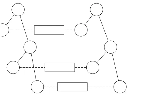
IfZ is rooted atr, then during an execution of [Π, A, Z], a singleinstance of Π will be running; ifZ is multi-rooted atr, then many instances of Π may be running. During the execution of such a system, it is helpful to visualize its dynamic call graph. The reader may wish to look at Fig. 2 on p. 24, which represents a dynamic call graph corresponding to two instances of a two-party protocol. In this figure, circles represent regular protocol machines. Rectangles represent ideal protocol machines, which are connected to their regular peers via a dotted line. In general, a dynamic call graph of regular machines will be a forest of trees, where the roots are the top-level machines that communicate directly with the environment.
Section 6: resource bounds
The main goal of this section is to define the notion of a polynomial time protocol.
When we define a polynomial time algorithm, we bound its running time as a function of the length of the input. For protocols that are reacting to multiple messages coming from an environment (either directly or via the dummy adversary), we shall bound the running time ofall the machines comprising the protocols as a function of thetotal length of all these messages.
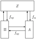
Z
Π A
fep
fap
fea
Figure 1: Flows
The execution of a system [Π, A, Z] will be driven by such a well-behaved environmentZ. The running time of the protocol will be bounded by the length of various flows:
• fep is the flow fromZ into Π;
• fea is the flow from Z into A;
• fap is the flow fromA into Π.
By flow, we mean the sum of the lengths of all relevant messages (including machine IDs and security parameter). To define the notion of a poly-time protocol, we do not need the flowfap, but this will come in handy later. See Fig. 1 for an illustration. We stress that in this figure, the box labeled Π represents all the running protocol machines.
Let us also define tp to be the total running time of all protocol machines running in the execution of [Π, A, Z], andta to be the total running time ofA in this execution.
Our definition of a poly-time protocol runs like this: we say a protocol Π rooted at r is (multi-)poly-time if there exists a polynomial psuch that for every well-behaved Z (multi-)rooted atr, in the execution of [Π, Ad, Z], we have
tp≤p(fep+fea)
with overwhelming probability. Recall thatAddenotes the dummy adversary. SinceAdis essentially a “wire”, observe that fap is closely related to fea.
Two points in this definition deserve to be stressed: (i) the polynomialpdepends on Π, but not onZ; (ii) the bound is required to hold only with overwhelming probability, rather than probability 1. We also stress that in bounding the running time of Π, we are bounding the total running time of all machines in Π in terms of the total flow out ofZ — nothing is said about the running time of an individual machine in terms of the flow into that machine.
This definition is really two definitions in one: poly-time (for “singly” rooted environments) and multi-poly-time (for “multiply” rooted environments). The main theorem in this section, however, states thatpoly-time implies multi-poly-time.
Section 7: emulation
all environments Z. Here, Exec[Π, A, Z] represents the output (which is generated by Z) of the execution of the system [Π, A, Z], and “≈” means “computationally indistinguishable”. Also, we quantify over all well-behaved environments Z, rooted at the common root of Π and Π1; if we allow multi-rooted environments, we say that Π1 multi-emulates Π, and otherwise, we say that Π1 emulates Π.
In the above definition, we still have to specify the types of adversaries, A and A1, over which we quantify. Indeed, we have to restrict ourselves to adversaries that are appropriately resource bounded.
Recall the above definitions of flow and running time, namely, fep,fea,fea,tp, andta. Suppose Π is a protocol rooted atr. We say that an adversaryAis(multi-)time-bounded for Π if there exists a polynomialp, such that every well-behaved environment Z (multi-)rooted at r, in the execution of [Π, A, Z], we have
tp+ta≤p(fep+fea)
with overwhelming probability. We also say that A is (multi-)flow-bounded for Π if there exists a polynomialp, such that every well-behaved environmentZ (multi-)rooted atr, in the execution of [Π, A, Z], we have
fap ≤p(fea) with overwhelming probability.
So in our definition of emulation, we restrict ourselves to adversaries that are both (multi-)time-bounded and (multi-)flow-(multi-)time-bounded — we call such adversaries (multi-)bounded. The time-boundedness constraint should seem quite obvious and natural. However, the flow-time-boundedness constraint may seem somewhat non-obvious and unnatural; we shall momentarily discuss why it is needed, some difficulties it presents, and how these difficulties may be overcome.
It is easy to see that if Π is (multi-)poly-time, then the dummy adversary is (multi-)bounded for Π. So we always have at least one adversary to work with that satisfies our constraints — namely, the dummy adversary — and as we shall see, this is enough.
We state here the main theorems of this section.
Theorem 5 (completeness of the dummy adversary) Let Π and Π1 be (multi-)poly-time protocols rooted at r. Suppose that there exists an adversary A that is (multi-)bounded for Π, such that for every well-behaved environment Z (multi-)rooted at r, we have Exec[Π, A, Z] ≈
Exec[Π1, Ad, Z]. Then Π1 (multi-)emulates Π.
Theorem 6 (emulates =⇒ multi-emulates) Let Π and Π1 be poly-time protocols. If Π1 emulates Π, then Π1 multi-emulates Π.
Recall that if a protocol is poly-time, then it is also multi-poly-time, so the statement of The-orem 6 makes sense. Because of these properties, we ignore multi-emulation in the remaining two theorems.
Theorem 7 (composition theorem) Suppose Π is a poly-time protocol rooted atr. Suppose Π0 is a poly-time subprotocol of Π rooted atx. Finally, suppose Π0
1 is a poly-time protocol also rooted atxthat emulates Π0 and that is substitutable for Π0 in Π. Then Π1 := Π[Π0/Π01] is poly-time and emulates Π.
The composition theorem (Theorem 7) is arguably the “centerpiece” of any universal composi-tion framework. It says that if Π0
1 emulates Π0, then we can effectively substitute Π01 for Π0 in any protocol Π that uses Π0 as a subprotocol, without affecting the security of Π.
It is in the proof of the composition theorem that we make essential use of the flow-boundedness constraint. This constraint allows us to conclude from the hypotheses that the instantiated protocol Π1 is itself poly-time. In order to use the composition theorem in a completely modular way, this is essential — typically, the protocol Π will be designed without regard to the implementation of Π0, and the protocol Π0
1 is designed without regard to the usage of Π0 in Π.
If we drop the flow-boundedness constraint, the composition theorem is no longer true, and in particular, Π1 may not be poly-time. Perhaps there is another type of constraint that would allow us to prove the composition theorem, but our investigations so far have not yielded any viable alternatives.
The flow-boundedness constraint can, at times, be difficult to deal with. Indeed, it turns out that in some situations, it is difficult to design a simulator that satisfies it. To mitigate these difficulties, we found it necessary to use a somewhat more refined notion of poly-time than that discussed above. The idea is to introduce the notion ofinvited messages: a protocol machine may invite the adversary to send it a specific message, and the adversary mayinvite the environment to send it a specific message. We then stipulate that such invited messages are ignored for the purposes of satisfying the flow-boundedness constraint; however, they are also ignored for the purposes of bounding running times. Formally, this simply amounts to defining fea and fap to count only uninvited messages.
Using this invitation mechanism, we may allow the adversary to send certain “control messages” to the protocol, “free of charge”, so to speak. Of course, the protocol designer must ensure that these invited messages do not upset the running-time bounds — this typically amounts to a very simple form of “amortized analysis”. Our main use of the invitation mechanism is in the treatment of corruptions.
In our analysis of the application of our framework to many known “use cases”, we have found that by using the invitation mechanism, along with a few simple design conventions, the flow-boundedness constraint does not present any insurmountable problems.
The flow-boundedness constraint may also seem to limit the adversary in a way that would rule out otherwise legitimate attacks — see Note 7.3 for a discussion on why this is not the case.
Section 8: Conventions regarding corruptions and ideal functionalities
Perhaps somewhat surprisingly, our fundamental theorems, such as the composition theorem, are completely independent of our mechanism for modeling corruptions, which is layered on top of the basic framework as a set of conventions. This section describes these conventions.
Basically, the environment may choose to corrupt a “top level” regular protocol machine by sending it a special corrupt message. When this happens, the chosen machine responds by notifying the adversary that it is corrupted. This notification may include some or all of the current internal state of the corrupted machine — this depends on whether one wants to model secure erasures or not.
graph rooted atM. Moreover, for each subroutine ofM extant at the time ofM’s corruption, the corresponding “subroutine corruption instructions” are invited messages, which means the adver-sary is free to carry out this recursive corruption procedure, without breaking the flow-boundedness constraint. Similarly, the adversary is invited to send an instruction toM that will causeM to send the special corruption message to its ideal peer — the behavior of the ideal peer upon receiving this message is entirely protocol dependent.
Our model of corruptions enforces a strict hierarchical pattern of corruption, so that if Q is a subroutine of P, and Q is corrupted, then P must be corrupted as well.
This section also includes the definition of an ideal protocol, which is a particularly simple type of protocol, for which a single instance of the protocol consists of just an ideal machine, along with regular peers, so-called “dummy parties”, that just act as “wires”, each of which connects the ideal machine to the caller of the dummy party. The logic of the ideal machine is called an ideal functionality.
We also define the notion ofhybrid protocols. IfF1, . . . ,Fkare ideal functionalities, then we say that a protocol Π is an (F1, . . . ,Fk)-hybrid protocol of the only non-trivial ideal machines used by Π are instances of theFi’s.
Section 9: protocols with joint state
Consider an F-hybrid protocol Π. Note that this means that even a single instance of Π can use multiple instances ofF. These subprotocol instances will be independent, and thus their potential implementations will also be independent — in particular, they may not share joint state. Thus, ifF represents, say, an authenticated channel, we will not be able to implement all these different
F-instances using, say, the same signing key.
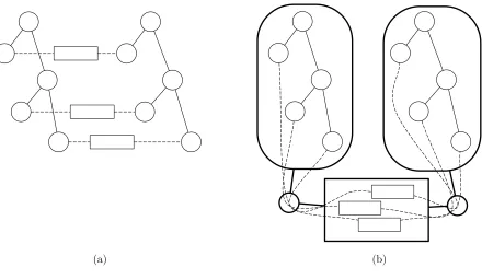
This section provides a construction and a theorem — the so-called JUC theorem [CR03] — that allows us to sidestep this issue. The basic idea is this. First, we transform F into its multi-session version Fb. Second, we transform Π into a “boxed” protocol [Π]F, in which all of the individual regular protocol machines that belong to one “party” will be run as virtual machines inside a single “container” machine, where calls to the various F-instances are trapped by the container, and translated into calls to a single running instance ofFb. Our JUC Theorem (Theorem 9) then states that [Π]F emulates Π.
Of course, this is only interesting if we can design a protocol Π that emulatesb Fb. For our example above, where F models an authenticated channel, this can be done in a straightforward way, assuming some kind of ideal functionalityFcawhich represents a “certificate authority”. Then applying ordinary composition and transitivity, we get aFca-hybrid protocol Π1 that emulates Π. This type of application is one of the main motivations for the JUC theorem — it allows us to replace a slow authenticated channel (i.e., between a user and a certificate authority) with a faster one (i.e., one based on signatures).
We note that unlike the composition theorem, the JUC theoremdoesdepend on our conventions regarding corruptions, and its proof relies in an essential way on the invitation mechanism.
Section 10: an extension: common functionalities
In this section, we present an extension to our framework, introducing the notion of common functionalities, which will involve some revisions to the definitions and theorems in the previous sections.
The goal is to build into the framework the ability for protocol machines that are not necessarily peers, and also (potentially) for the environment, to have access to a “shared” or “common” functionality.
For example, such a common functionality may represent a system parameter generated by a trusted party that is accessible to all machines in the system. By restricting the access of the environment, we will also be able to model a common reference string (CRS) — the difference being that a simulator is allowed to “program” a CRS, but not a system parameter. Using this mechanism, we can also modelrandom oracles, bothprogrammable and non-programmable.
We stress that our modeling of a CRS differs from the usual UC modeling, e.g., in [CF01]. Namely, [CF01] model a CRS as a hybrid ideal functionality, which means that every instance of a subprotocol gets its own CRS. Using the JUC theorem, it is then possible to (non-trivially) translate many instances of a protocol with individual CRSs into one instance of a multiple-use protocol that uses only one CRS [CR03]. We believe that our modeling of a CRS is more natural and direct, although one could of course formulate a CRS ideal functionality in GNUC.
Without some kind of set up assumption, such as a CRS, it is impossible to realize many interesting and important ideal functionalities [CF01]. Moreover, with a CRS, it is feasible to realize any “reasonable” ideal functionality [CLOS02] under reasonable computational assumptions. (While the results in [CF01] use a CRS that is formalized as a hybrid functionality, they also carry over easily to our CRS formalization.)
In contrast to CRSs, system parameters are not essential from a theoretical point of view, but often yield more practical protocols.
Section 11: comparison with UC05 and other frameworks
In this section, we compare our proposed UC framework with Canetti’s UC05 framework [Can05], and (more briefly) with some other frameworks, including K¨usters’ IITM framework [K¨us06], and the Reactive Simulatability framework of Backes, Pfitzmann and Waidner [BPW07].
Section 12: examples
In this section, we give some examples that illustrate the use of our framework. These examples include several fundamental ideal functionalities, carefully and completely specified in a way that is compatible with our framework. These examples also include a more detailed discussion of how the JUC theorem may be used together with a certificate authority to obtain protocols that use authenticated channels, and that are designed in a modular way within our framework, but yet are quite practical. Finally, the results in [BCL+05], on secure computation without authentication, are considered, and we discuss how these may be translated into our framework.
3
Machine models
3.1 Some basic notation and terminology
We assume a fixed programming language for writing programs; programs are written as strings over Σ. We assume that our programs have instructions for generating a random bit. We also assume that a program takes as input a string over Σ and outputs a string over Σ. For
π, α∈Σ∗, if we viewπ as a program andα as an input, the notationβ ←Eval(π, α) means that the program π is run on input α, and if and when the program terminates with an output, that output is assigned toβ. Ifω∈ {0,1}∞is an infinite bit string, we may also writeβ ←Eval(π, α;ω) to mean thatπ is run on inputα, usingω as the source of random bits, and the output is assigned toβ. When discussing the execution of such probabilistic programs, we are assuming a probability space on{0,1}∞ analogous to the Lebesgue measure on [0,1].
Finally, we assume a fixed list-encoding functionh · i: ifα1, . . . , αn are strings overΣ, then hα1, . . . , αni is a string over Σ that encodes the list (α1, . . . , αn) in some canonical way. It may
be the case that a string does not encode a list, but if it does, then that list must be unique. We assume the encoding and decoding functions may be implemented in polynomial time. We also assume that the length ofhα1, . . . , αni is at leastn plus the sum of the lengths ofα1, . . . , αn. For
example, one could define hα1, . . . , αni := |Quote(α1)|· · ·|Quote(αn), where Quote(α) replaces each occurrence of |inα with the “escape sequence”\|, and each occurrence of \with\\.
3.2 Interactive machines
An interactive machine (IM) M consists of a triple (id, π,state), where id is its machine ID, π is its program, and state is its current state, all of which are strings over Σ. Given id0,msg0 ∈Σ∗, the machineM computesγ←Eval(π,hid,state,id0,msg0i)∈Σ∗. The outputγ is expected to be of the formhstate0,id1,msg1i, for somestate0,id1,msg1∈Σ∗. Such a computation is called an activation of M.
At the end of such an activation , the current state of M is modified, so that now M consists of the triple (id, π,state0) — although the state of M changes, we still consider it to be the same machine (and the values of id and π will never change). Intuitively, msg0 represents an incoming message that was sent from a machineM0 with machine IDid0, whilemsg1 represents an outgoing message that is to be delivered to a machineM1 with machine ID id1.
We say that a program π is a valid IM program if the following holds: for all id,state,id0,msg0∈Σ∗, whenever the computationEval(π,hid,state,id0,msg0i) halts, its output is the encoding of a triple, that is, a string of the formhstate0,id1,msg1ifor somestate0,id1,msg1 ∈ Σ∗. Note that a valid IM program may be probabilistic, and may fail to halt on certain inputs and certain coin-toss sequences, but whenever it does halt, its output must be of this form.
Whenever we consider an IM, we shall always assume that its program is a valid IM program, even if this assumption is not made explicit. Note that while there is no algorithm that decides whether a given program π is a valid IM program, we can easily convert an arbitrary program π
into a valid IM program ¯π, which runs as follows: ¯π simply passes its input to π, and if π halts with an output that is a valid triple, then ¯π outputs that triple, and ifπ halts with an output that is not a valid triple, then ¯π outputs the tripleh h i,h i,h i i. Thus, ¯πacts like asoftware sandbox in whichπ is allowed to run. We will use this “sandboxing” idea extensively throughout the paper to make similar restrictions on programs.
To simplify notation, ifπ is a valid IM program, we express a single activation as
3.3 Machine models and running time
To complete our definition of an interactive machine, we should fully specify the programming language, the execution model, and the notion running time. However, as long as we restrict ourselves to models that are polynomial-time equivalent to Turing machines, none of these details matter, except for the specific requirements discussed in the next two paragraphs.
We assume that there is a universal programπu that can efficiently simulate any other program, and halt the simulation in a timely fashion if it runs for too long. To make this precise, define
B(π, α,1t, ω) to behbeepiif the running time of the computationβ ←Eval(π, α;ω) exceedst, and
hnormal, βi otherwise. The requirement is that Eval(πu,hπ, α,1ti;ω) computes B(π, α,1t, ω) in time bounded by a fixed polynomial in the length ofhπ, α,1ti.
We also assume that the programming language allows us to place a “comment” in a program, so that the comment can be efficiently extracted from the program, but does not in any way affect its execution. While not strictly necessary, this assumption will be convenient.
Finally, we define a simple notion of polynomial time for IMs. Let πbe an IM program. We say that π is multi-activation polynomial-timeif the following holds: there exists a polynomial p
such that for all
id,id0,msg0, . . . ,idk−1,msgk−1 ∈Σ∗, (1)
if
n:=|hid,id0,msg0, . . . ,idk−1,msgk−1i|,
then with probability 1, the following computation runs in time at mostp(n):
state ← h i fori←0 to k−1
hstate,id0i,msg0ii ←Eval(π,hid,state,idi,msgii)
In addition, if there is a polynomialq such that for all strings as in (1), we have|msg0i| ≤q(|msgi|)
fori= 0, . . . , k−1 with probability 1, we say that π isI/O-bounded.
3.4 Systems of interactive machines
Our next goal is to define a system of interactive machines. To do this, we first define two of the basic components of such a system.
The first basic component of such a system is a run-time library. This is a partial function Lib:Σ∗ →Σ∗ with a finite domain.
Intuitively, Lib maps program namesto programs (i.e., code). The definition implies that a given run-time library can only define a finite number of program names. The idea is that all programs for machines executing in a system of interactive machines will come from the run-time library. We writeLib(name) =⊥to mean that the given program namename is not in the domain of Lib.
The second basic component of a system of IMs is aname map. This is a functionNameMap: Σ∗ → Σ∗∪ {⊥} that can be evaluated in deterministic polynomial time. In addition, we require thatNameMap(h i) =⊥.
A given software libraryLiband name mapNameMapdetermine theprogram mapProgMap: Σ∗ → Σ∗ ∪ {⊥} defined as follows: for id ∈ Σ∗, if NameMap(id) = ⊥, then ProgMap(id) := ⊥, and otherwise, ifNameMap(id) =name 6=⊥, thenProgMap(id) :=Lib(name).
Intuitively, such a program map associates to each machine ID a corresponding program, or the symbol ⊥ if there is no such program. By definition, a program map can be evaluated in deterministic polynomial time.
A system of interactive machines (IMs) is a triple S = (idinit,NameMap,Lib), where idinit is a machine ID, NameMap is a name map, and Lib is a run-time library. We require that if ProgMap is the corresponding program map, then πinit:=ProgMap(idinit)6=⊥.
We shall next define the execution of such a system S. Such an execution takes an external inputα∈Σ∗, and produces anexternal outputβ ∈Σ∗, if the execution actually halts.
Intuitively, the execution of the system proceeds as a sequence of activations. The machine
Minit:= (idinit, πinit,h i) is theinitial machine, and it performs the first activation: starting with the (rather arbitrary) initial state h i, it is given the message hinit, αi, apparently originating from the “master machine”. In general, whenever a machineM performs an activation, it receives a message msg0 from a machine M0 with ID id0, and then M’s state is updated, and a message msg1 is sent to a machine M1 with ID id1, after which, the next activation is performed byM1. If there is no machineM1 with the IDid1, then a new machine is created afresh, using the program determined by the program map. Two special conditions may arise:
• id1 = h i (i.e., id1 is the ID of the “master machine”). In this case, the execution of the system terminates, and the output of the system is defined to be msg1.
• id1 6=h ibutProgMap(id1) =⊥(i.e., the program corresponding toid is undefined). In this case, a special error message (apparently originating from the “master machine”) is sent back toM.
We formalize of the above intuition by describing in detail the algorithm representing the execution of a systemS as above. To streamline the presentation, we make use of an “associative array” or “lookup table” Machine, which maps machine IDs to program/state pairs. Initially, Machine[id] =⊥ (i.e., is undefined) for all id ∈Σ∗; as the algorithm proceeds, for various values id, π,state, we will set Machine[id] to (π,state), so that the triple (id, π,state) represents an IM.
Input: α∈Σ∗ Output: β ∈Σ∗
id ←idinit; id0← h i; msg0 ← hinit, αi whileid 6=h i {
/∗ message msg0 is being passed from id0 to id ∗/
if Machine[id] =⊥
then {π ←ProgMap(id); state ← h i } // create new machine
else (π,state)←Machine[id] // fetch description of existing machine
/∗ perform one activation: ∗/
hstate0,id1,msg1i ←Eval(π,hid,state,id0,msg0i) Machine[id]←(π,state0) // update state
if id1 6=h i andProgMap(id1) =⊥
then {id0 ← h i;msg0 ← herror,id1,msg1i } // error – undefined program else {id0 ←id;msg0 ←msg1;id ←id1 } // pass message msg1 to id1
}
β ←msg0; output β
4
Structured systems of interactive machines
In the previous section, we defined the notion of a system of IMs. This is a very simple and general notion, but is far too general for our purposes. Our goal in this section is to define the notion of a structured system of IMs. It is with respect to such structured systems that our main theorems (such as the Composition Theorem) will be formulated.
In defining a structured system of IMs, we will define once and for all the name map (which maps machine IDs to program names) that will be used forall structured systems (although in§10 we will define the notion of an extended structured system, which will have some extra features). In addition, we will define various classes of machines that satisfy certain constraints — all of these constraints can be imposed “locally”, by software sandboxing, and we will not require any form of “global controller”, beyond the simple “master machine” that carries out the execution of a (general) system of IMs.
4.1 Some basic syntax
At a high level, in a structured system of IMs, there are three classes of machines: environment, adversary, andprotocol. Moreover, in any execution of a structured system, there will be only one instance of an environment machine, and only one instance of an adversary machine, so there will be no confusion when we speak of “the environment” and “the adversary”.
protocol machines whose machine IDs are peers are also called peers.
We next describe constraints on the format of PIDs and SIDs of protocol machines. We divide protocol machines into two subclasses: regular and ideal. These two subclasses of machines are distinguished by the form of their PIDs: regular machines have a PID of the formhreg,basePIDi, while ideal protocol machines have the PIDhideali. A typical PID of a regular machine could be of the form hreg,email addressi to denote machines associated with the party with a given email address.
As will be described in detail below, regular machines may invoke other regular machines as “subroutines”. When a machine P invokes a machine Q as a subroutine, we say that P is the caller of Q and Q is a subroutine of P. This caller/subroutine relationship will play a crucial role. An essential constraint we shall impose is the following:
every regular machine has a unique caller.
This is an important constraint, and we shall have much more to say about it. However, for the time being, we indicate how this constraint relates to the syntactic structure of SIDs.
SIDs for all protocol machines (regular and ideal) are structured as “path names”, which will be used to explicitly represent the caller/subroutine relationship of regular machines. That is, SIDs will be of the form
hα1, . . . , αki. (2)
Some terminology will be helpful. We say an SID sid0 is an extension of an SID sid if for some α1, . . . , α` ∈ Σ∗, and for some k ≤ `, we have sid = hα1, . . . , αki and sid0 = hα1, . . . , αk, αk+1, . . . , α`i. If` > k, we say sid0 is a proper extension of sid, and if `=k+ 1,
we saysid0 is aone-step extension ofsid.
Next, we define a simple syntactic relation on machine IDs. Given two machine IDs id =
hpid,sidi and id0 = hpid0,sid0i, we say that the ID id is a parent of the ID id0 if pid = pid0 and sid0 is a one-step extension ofsid. Evidently, the parent of any ID is uniquely determined. As usual, if id is a parent ofid0, then we also say that id0 is a child of id. Moreover, we say that id is anancestor of id0 ifpid =pid0 and sid0 is a proper extension of sid.
With this definition in hand, we can state more precisely the constraint that regular machines will satisfy: for any regular machine with ID id, its caller is either the environment or the regular machine whose ID is the parent of id. This will be more precisely formulated below.
For an SID of the form (2), the last component, namely, αk, is called the basename of the
SID. This basename also must be of a particular form, namely, hprotName,spi. Here, protName specifies the name of the program being executed by the machine. For protocol machines, we require that program names be of the form prot-name. We call a program name of this form a protocol name. Also, sp is an arbitrary string, which we call a session parameter — its contents is determined by the application.
To give an example, an SID for a zero-knowledge protocol (for a relation rel) that is called as a subroutine by a commitment protocol could be of the form h hprot-commit, hsender,receiver,labeli i,hprot-zk,hsender,receiver,rel,label’i i i. Here, sender and receiver de-note the PIDs of the corresponding peers, and label,label’ are labels that distinguish different instances of the same protocol.
That completes the description of the format of the machine IDs of protocol machines. Now that we have defined the format of all machine IDs, we can define the name map that will be used in every structured system of IMs. The name map will map the machine ID henvi to the program nameenv, the machine IDhadvito the program nameadv, and a machine ID of the form
Of course, certain aspects of this definition of the name map are somewhat arbitrary, but we have included them for specificity.
4.2 Overall execution pattern
We now describe the overall execution pattern of a structured system of IMs.
The environment is the initial machine. In any execution of the system, it will be given the external input and will perform the first activation.
In all executions of interest, the external input will be of the form 1λ, whereλ represents the security parameter. We will also insist on the following constraints:
C1: The environment is the only machine that can produce an external output (and thereby halt the execution of a structured system).
C2: Every message sent from one machine to another is of the form h1λ, m, i1, . . . , iki, where λis
the security parameter; m is called themessage body, and i1, . . . , ik are calledinvitations; invitations may be included only in messages from a protocol machine to the adversary, and in messages from the adversary to the environment.
Note that there is no constraint placed on the format of the external output generated by the environment.
These constraints are easily enforced by sandboxing. To implement constraint C1, the sandbox would check for an illegal attempt to generate an external output — if this happens, the message would simply be sent to the adversary (this will always be legal). Similarly, if a machine generates a message that does not satisfy constraint C2, the message is translated into one that does; the details of this translation are not so important, but we can assume that the message is simply replaced byh1λ,h i i.
Invitations will play a special role when we discuss running time and other resource bounds in
§6 and §7. For now, we leave the reader with the following, admittedly vague, intuition: when a machine P sends an invitation ito a machine Q, this is a hint that Q should send the message i
back toP.
Because the security parameter is always transmitted as part of a message, when describing pro-tocols at high level, we will generally leave the security parameter out of the description. Whenever we say “send messagem”, the low-level message that is transmitted is actuallyh1λ, mi. Whenever we say “send message m with invitations for i1, . . . , ik”, the low-level message that is transmitted
is actually h1λ, m, i1, . . . , iki.
4.3 Constraints on the environment
In addition to the constraints imposed in§4.2, we shall impose additional constraints on the envi-ronment.
C3: The environment may send messages to the adversary, and may send messages to regular protocol machines; however, it may notsend messages to ideal protocol machines.
Constraint C4 can be rephrased as saying that among the regular protocol machines to which the environment sends messages, no one machine may have an SID that is a proper extension of the SID of any other machine. These constraints are easily enforced by sandboxing.
Note 4.1. Constraint C4 is not necessary to prove any of the theorems in this paper. However, this constraint can be justified, and including it helps to justify some other constraints — see Note 8.10.
Note 4.2. The set of constraints taken together will imply that the only machines from which the environment receives messages are the adversary and the regular protocol machines to which it has already sent a message.
Note 4.3. If the environment specifies an SID of the form hα1, . . . , αki, we do insist that αk is
a well-formed basename; however, we do not make any other constraints: the program name need not be specified by the library, and α1, . . . , αk−1 may be completely arbitrary strings.
4.4 Constraints on the adversary
In addition to the constraints imposed in §4.2, we shall impose an additional constraint on the adversary:
C5: The adversary may send messages to the environment. The adversary may send a message to a protocol machine (regular or ideal) only if it has previously received a message from that machine.
Again, this constraint is easily enforced by sandboxing.
Note 4.4. This constraint means that the adversary never causes a protocol machine to be created.
Note 4.5. The set of constraints taken together will imply that the adversary may receive messages from the environment and from any existing protocol machine (regular or ideal).
Note 4.6. Constraint C5 may seem like an unrealistic restriction, since we normally think of the adversary as being generally unfettered. However, this constraint could alternatively be imposed by constraining protocol machines, so that messages received from the adversary too early would simply be ignored and bounced back to the adversary. Thus, this constraint may be viewed as a constraint on the protocol, rather than the adversary.
4.5 Constraints on ideal protocol machines
In addition to the constraints imposed in §4.2, we shall impose an additional constraint on ideal protocol machines:
C6: The only machines to which an ideal protocol machine may send messages are (i) the adversary and (ii) regular peers of the ideal machine from which it has previously received a message.
Again, this constraint is easily enforced by sandboxing.
4.6 Constraints on regular protocol machines
In addition to the constraints imposed in §4.2, we shall impose additional constraints on regular protocol machines. These constraints will require sandboxing — not only to enforce certain behav-ior, but to structure the computation in a particular way. Thus, we will insist that the program of the machine is structured as an “inner core”, which is running inside a “sandbox”. The inner core is quite arbitrary; however, the sandbox is fully specified here.
Let us call this regular machine M, and suppose id is its machine ID. Let parentId be the machine ID that is the parent ofid. Because of all the constraints we are imposing across the system, the first message received by M (and the one that brings it into existence) will be from either the environment or a regular protocol machine with ID parentId; moreover, whichever machine sends this first message, the other machine will never send it a message. We call the machine sending this first message the caller of M, and let us denote it here by C. We will also say that C invokes
M.
4.6.1 Caller ID translation
The first function of the sandbox is “caller ID translation”, which works as follows:
C7 (caller ID translation): When M receives a message from C, then if C is the environment, the sandbox changes the source address of the message to parentId before passing the message for further processing to the inner core. Similarly, when the inner core generates a message whose destination address is parentId , and C is the environment, then the sandbox sends the message instead to the environment.
To implement caller ID translation, the sandbox will have to store the true identity of C; however, this information will never be directly accessible to the inner core. This can be achieved by structuring the state ofM to be of the formhsandboxState,coreStatei, and only passingcoreState to the inner core.
Note 4.8. Caller ID translation is useful in that it effectively hides the true identity of caller of
M, which will be crucial in proving the main composition theorem.
4.6.2 Communication constraints
The second function of the sandbox will be to enforce constraints on the machines to whichM may send messages.
C8 (communication constraints): M is only allowed to send messages to the following ma-chines:
• the adversary;
• its ideal peer;
• machines whose machine IDs are children of id ;
• the caller of M, via caller ID translation — the inner core is not allowed to address a message directly to the environment.
4.6.3 Subroutine constraints
In§4.6.2, we allowedM to send messages to machines whose IDs are children ofid. Such a machine
S is called a subroutine of M. Because of all the constraints we have imposed, M must in fact be the caller of S, i.e., the first machine to send a message to S and to bring it into existence.
We shall require that M’s program explicitly declares the program names of any subroutine it may invoke during any activation. As we are assuming that a “comment” can be placed in a program (see §3.3), this declaration can be placed in the program as a “comment”, using any convenient format to encode the declaration. This could also be achieved by modifying the notion of a library, so that it allows us to associate such “comments” with the program, instead of embedding them in the program itself. The details are really not important. Let us call this declaration the subroutine declaration of M.
We require, of course, that the sandbox actively enforces the subroutine constraints:
C9 (subroutine constraints): M only invokes subroutines whose program names are explicitly declared in its subroutine declaration.
Note 4.9. The set of all constraints taken together will imply that a regular protocol machine will receive messages only from its caller, its ideal peer (unique, if it exists at all), its subroutines (if any), and the adversary.
Note 4.10. Regular and ideal protocol machines with a given program differ only in their PID. Thus, the various constraints for ideal and regular protocol machines will be enforced by a single sandbox — the behavior of this sandbox will be determined by the format of the PID.
4.7 The dummy adversary
The dummy adversary is a special adversary that essentially acts as a router between the environ-ment and protocol machines. It works as follows:
• if it receives a message of the form hid, mi from the environment, and it has previously received a message from a protocol machine with machine ID id, then it sends m to that protocol machine; otherwise, it sends the messageherrori back to the environment;
• if it receives a messagem from a protocol machine with machine IDid, it sends the message
hid, mi to the environment;
• if it receives a message m along with invitations for i1, . . . , ik (see §4.2) from a
proto-col machine with machine ID id, it sends the message hid, mi along with invitations for
hid, i1i, . . . ,hid, iki to the environment.
That completely specifies the logic of the dummy adversary. We denote the dummy adversary by Ad.
Intuitively, a message hid, mi is an instruction to the dummy adversary to send the message
5
Protocols
5.1 Definition of a protocol
We next define what we formally mean by aprotocol. A protocol is a run-time library that satisfies the following four requirements.
P1: The library should only define programs for protocol names. In particular, a protocol does not define the program for the environment or the adversary.
P2: The programs defined in the library should satisfy all the constraints discussed in§4 that apply to protocol machines.
Before we state the next requirement, recall that the subroutine constraint (C9) in §4.6.3 says that the program for a regular protocol machine must explicitly declare the program names of the machines it is allowed to invoke as subroutines during any activation.
P3: For each program name defined by the library, every program name declared by its correspond-ing program must also be defined by the library.
Before we state the last requirement, we need to define the static call graphof the protocol. The set of nodes of this graph is the domain of the library, that is, the set of protocol names defined by the library; there is an edge from one program name to another if the subroutine declaration in the program associated with the first name allows a call to the second (by requirement P3, the second name is defined by the library, and so is a node in the graph).
P4: The static call graph is acyclic and has a unique node of in-degree 0.
The noderdefined in P4 is called therootof the protocol — we may also say that the protocol is rooted at r. It follows from the definition that every node in the static call graph is reachable from r.
5.2 Subprotocols
We next define what it means for one protocol to be a subprotocol of another. The definition is quite natural, and is easy to define in a simple, mathematically rigorous way, as follows.
Let Π and Π0 be protocols, as defined in§5.1 Recall that these are functions with finite domains, say,Dand D0. We say that Π0 is a subprotocol of Π ifD0 ⊂Dand the restriction of Π to D0 is equal to Π0.
Let Π be a protocol which defines a protocol namex. LetD0 be the set of nodes reachable from
x in the static call graph of Π. Let Π0 be the restriction of Π toD0. Then it is easy to see that Π0 is a subprotocol of Π with root x. We call Π0 thesubprotocol of Π rooted at x, and we denote it by Π|x.
It is clear that if Π0 is an arbitrary subprotocol of a protocol Π, then Π0 = Π|x for somex.
Now, let Π0 := Π | x, and let Π0
1 be any other protocol rooted at x. We say that Π01 is substitutable for Π0 inΠ if the following condition holds: for everyy in the domain of Π\x, ify is also defined by Π01, then the definition of y in Π01 agrees with that in Π. If this condition holds, we write Π[Π0/Π0
1] to denote the protocol Π1 rooted atr such that Π\x= Π1\x and Π1 |x= Π01. It is easy to see that Π1 exists and is uniquely determined. In words, Π[Π0/Π01] is the protocol obtained by substituting Π01 for Π0 in Π.
The substitution operation is symmetric. Specifically, the following is easy to prove: if Π01 is substitutable for Π0 in Π, and if Π
1 := Π[Π0/Π01], then it holds that Π0 is substitutable for Π01 in Π1, and that Π = Π1[Π01/Π1].
5.3 Protocol execution
Let Π be a protocol with root r. Let Z be a program defining an environment, meaning that it satisfies the constraints discussed in§4.2 and§4.3. that apply to the environment. IfZ only invokes machines with the same SID with protocol name r, we say that Z is rooted at r — note that in this case, Z trivially satisfies Constraint C4 in §4.3. IfZ invokes machines whose SIDs are not necessarily the same, but still all with protocol namer, we say that Z is multi-rooted at r.
For the remainder of this section, we assume that Π is a protocol rooted at r, and that Z is an environment multi-rooted at r. Also, we assume that A is a program defining an adversary, meaning that it satisfies the constraints discussed in§4 that apply to the adversary. The protocol Π, together withA and Z, define a structured system of IMs, which we denote [Π, A, Z].
For a given value of the security parameter λ, we may consider the execution of the system
[Π, A, Z] on the external input 1λ. This execution is a randomized process that may or may not
terminate.
For such an execution of [Π, A, Z], we may define the associated dynamic call graph, which evolves during the execution. At any point in time, the nodes of this graph consist of all regular protocol machines created during the execution up to that point. There is an edge from one machine to a second machine if the second is a subroutine of the first.
By our constraints on structured systems, this graph is a forest of trees, where the roots of these trees are precisely the machines directly invoked byZ; all the nodes in any one tree have the same PID; moreover, for any two nodes in this graph, if these two nodes are peers, then the roots of their respective trees are also peers.
In this graph, we may group together all those nodes belonging to trees whose roots are peers; let us also add to such a group any ideal machines that are peers of these nodes. Let us call such a grouping of machines an instance of Π. By the observations in the previous paragraph, every protocol machine in the system (regular or ideal) belongs to a unique instance. In addition, we may associate with each instance the common SID of the root nodes belonging to that instance. We call this the SID of the instance. In any one instance, all machines will have SIDs that are extensions of the SID of the instance.
IfZ is rooted atr, then there will only be one instance. IfZ is multi-rooted atr, there may be many instances. Constraint C4 says that for every two distinct instances, the SID of one cannot be an extension of the SID of the other. The total number of instances will be bounded by the number of messages thatZ sends to any protocol machine.
Figure 2: A dynamic call graph
(belonging to any instance), or back to Z (which, again, ends the epoch). The total number of epochs is bounded by the number of messages that Z sends to a protocol machine or to the adversary.
See Fig. 2 for a visual representation of a simple dynamic call graph corresponding to two instances of a two-party protocol. In this figure, circles represent regular protocol machines. Rect-angles represent ideal protocol machines, which are connected to their regular peers via a dotted line.
6
Resource bounds
In this section, we discuss various notions of resource bounds, including a definition of a polynomial-time protocol.
Suppose Π is a protocol rooted atr,Z is an environment multi-rooted atr, andAis an arbitrary adversary. Suppose we fix the value of the security parameterλ, and consider the execution of the structured system [Π, A, Z] on external input1λ
We wish to define several random variables which measure the running time of various ma-chines during this execution. To this end, TimeZ[Π, A, Z](λ) denotes the running time of Z,
TimeA[Π, A, Z](λ) denotes the running time of A, and TimeΠ[Π, A, Z](λ) denotes the sum of the
running times of all protocol machines. For convenience, we define
TimeΠ,A[Π, A, Z](λ) := TimeΠ[Π, A, Z](λ) + TimeA[Π, A, Z](λ).
We also wish to define several random variables which measure the amount of flow of data between various machines during this execution.
For the purposes of this definition, we measure the length of a message from one machine to another as the length of the stringhid,id0,msg0i, whereid is the machine ID of the recipient,id0 is the machine ID of the sender, and msg0 is the low-level message, which is of the form h1λ, . . .i, as discussed in§4.2.
We also need to distinguish between invited messages and uninvited messages. Recall that messages from A toZ, and messages from a protocol machine to A, may include invitations (see