Computational Aspects of 2D-Quasi-Periodic-Green-Function
Computations for Scattering by Dielectric Objects
via Surface Integral Equations
Pieter Jorna*, Vito Lancellotti, and Martijn C. van Beurden
Abstract—We describe a surface integral-equation (SIE) method suitable for computation of electromagnetic fields scattered by 2D-periodic high-permittivity and plasmonic scatterers. The method makes use of fast evaluation of the 2D-quasi-periodic Green function (2D-QPGF) and its gradient using a tabulation technique in combination with tri-linear interpolation. In particular we present a very efficient technique to create the look-up tables for the 2D-QPGF and its gradient where we use to our advantage that it is very effective to simultaneously compute the QPGF and its gradient, and to simultaneously compute these values for the case in which the role of source and observation point are interchanged. We use the Ewald representation of the 2D-QPGF and its gradient to construct the tables with pre-computed values. Usually the expressions for the Ewald representation of the 2D-QPGF and its gradient are presented in terms of the complex complementary error function but here we give the expressions in terms of the Faddeeva function enabling efficient use of the dedicated algorithms to compute the Faddeeva function. Expressions are given for both lossy and lossless medium parameters and it is shown that the expression for the lossless case can be evaluated twice as fast as the expression for the lossy case. Two case studies are presented to validate the proposed method and to show that the time required for computing the method of moments (MoM) integrals that require evaluation of the 2D-QPGF becomes comparable to the time required for computing the MoM integrals that require evaluation of the aperiodic Green function.
1. INTRODUCTION
Reliable prediction of the interaction of electromagnetic fields with periodic structures plays a key role in numerous applications whether it is in the radio-frequency (RF) regime or in the optical regime. In the RF regime, periodic structures are for instance used to model the scattering properties of large arrays and frequency-selective surfaces. In the optical regime, an application of great importance is the scattering of light by diffraction gratings. To enable accurate and efficient computation of fields scattered by periodic structures, considerable effort has been invested over the years in the development of a range of numerical methods. For many of these methods the performance is excellent as long as the periodically repeated scattering objects have low contrast, but for high permittivity and plasmonic scatterers the problem of obtaining sufficiently accurate results in acceptable computation times arises often. In the RF regime, metals can mostly be modeled by PEC structures but in the optical regime they exhibit plasmonic behavior, see [1] and [2], hence in the optical regime the problem of dealing with plasmonic scatterers is especially important.
While the very successful Finite Element Method (FEM) and Volume Integral-Equation (VIE) method apply a volumetric discretization, the Surface Integral Equation (SIE) formulation only uses
Received 17 July 2015, Accepted 4 October 2015, Scheduled 19 October 2015 * Corresponding author: Pieter Jorna ([email protected]).
the unknown electromagnetic field on the boundaries of the object domains by introducing equivalent electric and magnetic surface current densities. These equivalent current sources on the boundaries yield an accurate representation of the fields in the interior and the exterior of the objects via exact Green function expressions. The SIE method therefore does not need to discretize the fields inside the object volumes but only applies a discretization of the surface current densities on the boundaries. This is especially advantageous in the case of high contrast and metal objects for which an accurate representation of the fields in the interior via discretization is often difficult to realize. It is for this reason that we have developed an efficient SIE method for the computation of electromagnetic fields scattered by 2D-periodic structures in 3D space.
We restrict the class of problems to the computation of electromagnetic fields scattered by an arbitrary number of mutually disjoint 2D-periodically repeated penetrable objects in a 3D homogeneous space. This is in itself an important class of problems but it is also of vital importance in the more complex application in which the 2D-periodically repeated objects are embedded in a multilayered medium. In the latter application the Green function has a spectral representation and a typical strategy for acceleration involves identifying and extracting the asymptotic terms in the spectral sums, see [1, 3–6]. The extracted terms are computed separately and are added back to the spectral sums. For several of the components of the Green function the extracted terms correspond to a 2D-periodic array of sources in an infinite homogeneous medium and can therefore be computed with a method as the one described in this paper. An implementation that allows the penetrable objects to be connected and/or the inclusion of one object by another requires a similar adaptation as is needed for an aperiodic SIE formulation, see [7] and [8]. In addition, the method can be extended to incorporate scattering objects of infinite lateral extent that cross the periodic boundaries. This extension requires the use of overlapping basis functions along one edge of the unit cell to allow the equivalent currents to flow from one cell to the next, for detailed information see for instance [9–11].
grid can be and hence there is a trade-off between the required interpolation time and tabulation time and storage. We show that tabulation of the regularized QPGF and its gradient in combination with simple tri-linear interpolation may still only require limited tabulation time and storage but that it leads to a very significant reduction in the required computation time, by a factor of 100 times or more. For configurations with many unknowns, conventional MoM may no longer suffice and it becomes necessary to resort to fast algorithms as presented in [16] and [17] but both these algorithms can again benefit from the proposed efficient tabulation technique.
The paper is organized as follows. In Section 2 we start with a detailed description of the problem of interest. In Section 3, we briefly present the used SIE formulation. In Section 4 we address some important differences in the periodic SIE-formulation when compared to an aperiodic SIE-formulation. In Section 5 we present the Ewald representation of the QPGF and its gradient in terms of the Faddeeva function. In Section 6 we describe an efficient technique to compute the QPGF and its gradient by applying a combination of tabulation and interpolation. In Section 7 we present numerical results for two different configurations that serve to validate the proposed approach and demonstrate its efficiency. Finally, in Section 8 we conclude by summarizing the contributions of this paper.
2. FORMULATION OF THE PROBLEM
The problem statement is now described in detail and the notation used in the remainder of the paper is given. We are interested in being able to compute the electromagnetic field scattered by 2D-periodic structures in 3D space for a plane-wave incident field. In our modeling we assume 2D periodicity in 3D space with the periodic directions orthogonal to ˆz but not necessarily orthogonal to each other. The corresponding unit cell can then be described by a so-called Bravais lattice spanned by the primitive lattice vectors a1 and a2 lying in thexy-plane. Here we define the 2D unit cell U0 =U(0,0) with surface areaA=|a1×a2|as
U0=
x1a1+x2a2
x1, x2∈
−1 2,
1 2
. (1)
A 3D unit cell U3D
0 may be obtained by extending the 2D unit cell U0 to infinity in the negative and
positive z-direction. Any of the other cellsU3D
n =U(3Dn1,n2) with n1, n2 ∈ Z is obtained by translating the 3D unit cell with respect to the lattice vector an =a(n1,n2) =n1a1 +n2a2. The implementation described here allows the unit cell to contain a finite number of dielectric objects that are mutually disjoint and that are all embedded in a homogeneous background medium. Let us assume that we have
Q scattering objects in the unit cell U03D. We denote the domains occupied by these Q scatterers by
Dq withq ∈ {2, . . . , Q+ 1}and let ∂Dq be the (piecewise) smooth boundaries that enclose the domains
Dq. Note that we have not yet defined D1 as we have preserved this notation for the unit-cell space exterior to the scatterers. The boundary∂D1 of the domainD1 is assumed to comprise the boundaries that enclose the domains Dq with q ∈ {2, . . . , Q+ 1}, that is, ∂D1 = ∂D2∪. . .∪∂DQ+1. The latter definition implies that we do not include the cell boundary in ∂D1. We denote the unit normal vector on the boundary ∂Dq pointing outward from the domain Dq by ˆnq. For each of the Q+ 1 domains
Dq withq ∈ {1, . . . , Q+ 1} we take εq andμq to be the homogeneous permittivity and permeability of
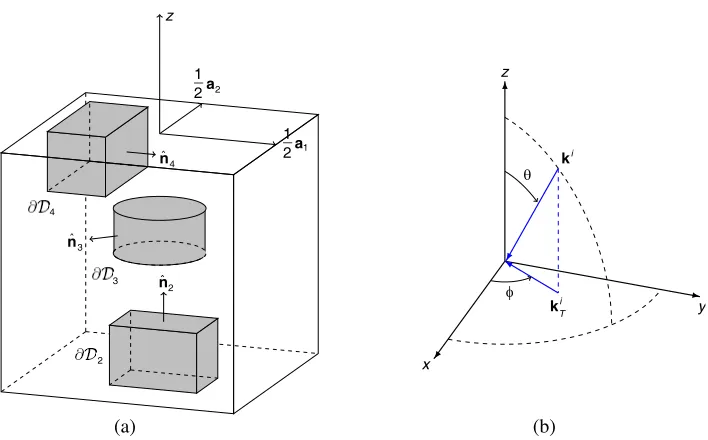
the domain. An example of a unit-cell configuration with three objects is given in Figure 1(a). In the figure, the unit cell is truncated in thez-direction such that it just contains all objects. In the following we denote observation points by r and source points by r. The vector pointing from source point to observation point is denoted byR=r−r= (rT+zˆz)−(rT+zˆz) =rT−rT+ (z−z)ˆz=RT+ (z−z)ˆz. The vector pointing from the shifted source pointr+an to observation pointris denoted byRn, that is,Rn =r−r−an=R−an.
We assume a plane wave of angular frequencyω is incident on the periodic structure under polar and azimuthal angles (θ,φ), defined with respect to the z- and x-axis, as is indicated in Figure 1(b). For ejωt time convention, the electric field belonging to such an excitation in the upper half space is given by
(a) (b)
ˆ ˆ
ˆ
1 2 1
2 z
n2 3
n
a2
a1 4
n
z
x
y
ki
T ki
θ
φ
4
3
2
Figure 1. Plane wave incident field impinging on a 2D-periodic configuration. (a) Unit-cell configuration with 3 objects. (b) Definition of the incident field direction of the impinging plane wave.
where
ki = −ω√ε1μ1(sinθcosφxˆ+ sinθsinφyˆ+ cosθˆz) (3)
= kiT +kizˆz and kiT =kixˆx+kiyyˆ, (4)
ˆs = −sinφˆx+ cosφyˆ, (5)
ˆ
p = cosθcosφxˆ+ cosθsinφyˆ−sinθˆz. (6) In these expressions, ki is the incident wave vector specifying the direction of the wavefront. The complex amplitudes along thes- andp-polarized directions of the incident electric field are denoted by
Es and Ep. Let b1 and b2 in the xy-plane be the reciprocal primitive vectors that satisfyai·bj =δij for i, j = 1, 2, with δij the Kronecker delta. Spectral representations of the quasi-periodic functions that we encounter in our analysis use the following set of points ink-space on the Bravais-lattice
kmT =kiT + 2πm1b1+ 2πm2b2, (7) with m = (m1, m2) and m1, m2 ∈ Z. Let k = ω√με be the wave number of the medium under consideration at angular frequencyω. Given the transverse component of the wave vectorkmT as defined in (7) the z-component of the complex propagation vector equals
γzm =
kmT ·kmT −k2. (8)
3. SIE FORMULATION 2D-PERIODIC DIELECTRIC STRUCTURES IN 3D SPACE
In the Surface Integral-Equation (SIE) method the unknown electric and magnetic fields in each of the domainsDq are fully determined by the prescribed sources in the domain Dq and by equivalent electric and magnetic surface-current densities on the boundary of the object domain. Since the domainsDqwith
q∈ {2, . . . , Q+ 1} represent scatterers and do not contain any sources, the only source is to be found in theD1 domain. The sources insideD1 are taken into account by imposing a plane-wave incident electric and magnetic fieldEi1(r) andHi1(r) as is described in the previous section. The equivalent electric and magnetic surface-current densitiesJq andMq at an arbitrary pointr ∈∂Dq on the boundary of object Dq are given by
Jq(r) = (Hq×nˆq) (r), (9)
and as such are again expressed in terms of the unknown electric and magnetic field at the boundary of the object. In this way we may obtain an Electric Field Integral Equation (EFIE) and a Magnetic Field Integral Equation (MFIE) for the domain boundary∂Dq by approaching the boundary from withinDq and taking the limit to the surface. For the same boundary ∂Dq we may obtain a second EFIE and MFIE by approaching the boundary from the other side, that is, from within D1 and taking the limit to the surface.
Here, we will use the well-known PMCHWT-formulation, named after Poggio, Miller [18], Chang, Harrington [19], Wu and Tsai [20], in which a first equation is obtained by subtracting the two EFIEs and a second equation is obtained by subtracting the two MFIEs. The PMCHWT-formulation imposes the following pair of coupled integral equations for each of the boundaries∂Dq withq∈ {2, . . . , Q+ 1}
−nˆq×E1i(r) =Zq(ˆnq×LqJq) (r)+(ˆnq×KqMq) (r)+ Q+1
p=2
(Z1(ˆnp×L1Jp) (r)+(ˆnp×K1Mp) (r)), (11)
−nˆq×Hi1(r) =Yq(ˆnq×LqMq) (r)−(ˆnq×KqJq) (r)+ Q+1
p=2
(Y1(ˆnp×L1Mp) (r)−(ˆnp×K1Jp) (r)), (12)
with, for q ∈ {1, . . . , Q+ 1}, Zq, Yq the wave impedance and the wave admittance of domain Dq and Lq,Kq the linear boundary integral operators that act on a surface-current density Xq on ∂Dq, defined as follows
(LqXq) (r) = jkq
∂Dq
Gqr,rXqrdA− 1 jkq∇
∂Dq
Gqr,r ∇S·XqrdA, (13)
(KqXq) (r) =
∂Dq
Xqr× ∇Gqr,rdA, (14)
where kq =ω√μqεq is the wave number of domainDq. In the operator definitions (13) and (14) G1 is the QPGF for an unbounded homogeneous space with the medium parameters of domain D1, i.e.,
G1
r,r= 1 4π
n∈Z2
e−jkTi·ane
−jk1|Rn|
|Rn| , (15)
whereasGqforq∈ {2, . . . , Q+ 1}is the aperiodic scalar Green function for an unbounded homogeneous space with the medium parameters of domainDq, i.e.,
Gqr,r= e
−jkq|r−r|
4π|r−r|. (16)
4. IMPORTANT DIFFERENCES APERIODIC AND PERIODIC SIE-FORMULATION
We use the Method of Moments (MoM) technique [21] to solve the coupled set of equations. In this procedure the equivalent surface-current densities are expanded in terms of Rao-Wilton-Glisson (RWG) basis functions [22], and Eqs. (11) and (12) are tested with ˆn×RWG test functions, see also [10]. To determine the matrix elements of the MoM matrix, we apply a singularity-extraction of the static Green function when source and observation point are nearby. The singular part is integrated analytically and the regular remainder is integrated via Gaussian quadrature.
x1
x2
z
(a) (b)
(c) (d)
x1
x2
x2
x2
x2
x1
x1
x1
-2Δφ -Δφ Δφ 2Δφ
-2Δφ -Δφ Δφ 2Δφ
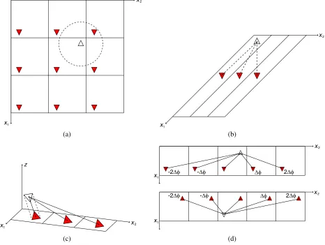
Figure 2. Test triangle (open) and source triangles (solid) in the same cell and neighboring cells: (a) Orthogonal lattice vectors. (b) Non-orthogonal lattice vectors. (c) Contributions to the gradient of the QPGF. (d) Interaction of source triangles (solid) and test triangle (open) with a progressive phase modulated onto the periodically repeated sources.
In Figure 2(b) it is shown that in the latter case the nearest source triangle may not even be located in one of the neighboring cells of the original unit cell.
To evaluate the surface integrals that arise from testing theKq operator, defined in (14), with RWG test functions after having expanded the current densities using RWG basis functions, we make use of the expression for the gradient of the Green function. The property that the gradient of the aperiodic Green function, defined in (16), is always pointing in the radial directionr−r is often explicitly used in the integration routine. In particular, it is used that the surface integral is zero in case the source and test triangle are located in the same plane. It is important to note that the gradient of the QPGF is no longer pointing in the radial directionr−r due to the contributions of the source triangles outside the unit cell as is illustrated in Figure 2(c). In the 2D-periodic case, the surface integral for a source and test triangle in the unit cell located in the same plane is no longer guaranteed to be zero except when the plane is parallel to or coincides with thexy-plane.
symmetry properties still apply to the Periodic Green Function (PGF), not all of the properties hold for the QPGF. The QPGF is symmetric for the interchange of variableszandzbut not for the interchange of variablesrT andrT. It is the phase modulated onto the periodically repeated sources in the transverse plane that breaks the symmetry. Figure 2(d) illustrates that the role of expansion and test function cannot simply be interchanged due to the progressive phase added to the sources.
Other than suggested in [10, Section 2] and in [14,§3], the QPGF with the variables rT and rT
interchanged cannot be obtained by computing the complex conjugate of the original QPGF. In Section 5 we will however show that the additional work necessary to compute the QPGF forr−rwhile computing the QPGF forr−r is minimal and hence simultaneous computation of the QPGF forr−rand r−r
can be made very efficient.
5. QUASI-PERIODIC GREEN FUNCTION AND THE EWALD TRANSFORMATION
Key to the feasibility of the SIE method for 2D-periodic structures is an efficient evaluation of the QPGF and its gradient. The spatial representation of the 2D QPGF is a double-infinite series in which the contributions of all 2D-periodic source points are summed with the proper phase, i.e.,
GspatialΛ = 1
4π n∈Z2e −jki
T·ane−jk|Rn|
|Rn| . (17)
In very lossy media and in metals that exhibit plasmonic behavior, this spatial series expression yields an efficient way of computing the 2D-QPGF and its gradient as only a limited number of terms is required in the summation since the amplitude of the terms decays exponentially with |Rn|. In a lossless background medium (such as air), however, these series exhibit very slow convergence since the amplitude of the terms in the summation only decays with 1/|Rn|. An alternative method of computing the 2D-QPGF and its gradient may be provided by using the spectral representation of the 2D QPGF, a 2D quasi-periodic Fourier series that sums the contributions of all 2D quasi-periodic Fourier modes
GspectralΛ = 1 2A
m∈Z2
e−jkmT·RTe−γ
m
z |z−z|
γzm . (18)
For observation points at a heighth=z−zwell above or below the source point, the contributions of the evanescent modes decay exponentially with Re{γzm} and the spectral representation of the 2D-QPGF and its gradient is very efficient. For this reason we use the spectral representation of the 2D-QPGF and its gradient to compute the reflection and transmission coefficients. This double series, however, has convergence problems if the point of observation is located at (approximately) the same height as the source point.
To solve the convergence problems we may use the Ewald representation for the QPGF. In the Ewald representation, the QPGF is split up into the sum of a modified spatial and a modified spectral series using the so-called splitting parameterE, i.e.,
GΛ,E =
n∈Z2
GspatialΛ,E,n +
m∈Z2
GspectralΛ,E,m . (19)
Both the spatial and spectral series part of the Ewald representation of the QPGF possess Gaussian decay regardless of the loss properties of the medium and the height h =z−z between observation and source point. The splitting parameter E is an arbitrary number but in [13] an optimal value
Eopt = π/A is derived that balances the convergence rate of both series, thereby causing the total number of terms needed for the calculation to be minimized. In [23], it has been shown that values ofE
is remedied by requiringk2/(4E2) < H2 where H2 is the maximum exponent permitted, which in the articles is taken to beH2= 9. We have used this simpler approach and for general complex k we take
E = max
Eopt, Re{k}
2H
. (20)
While there are various ways of presenting the Ewald representation of the QPGF, most often the Ewald representation of the QPGF is given in terms of the complementary error function. For complex arguments the complementary error function can be computed using the scaled complex complementary error function, i.e., the Faddeeva function w(z), see [27], as
erfc (z) =e−z2w(jz). (21)
In practice it is not efficient to actually compute the complementary error function after having evaluated the Faddeeva function. Instead, we use the Ewald representation of the QPGF in terms of the Faddeeva function w(z). The terms in the modified spatial series and the modified spectral series are given by
GspatialΛ,E,n =
e−jkiT·an−(|Rn|E)2+(2kE)2 8π|Rn|
w
j|Rn|E− k
2E
+ w
j|Rn|E+ k 2E
, (22)
GspectralΛ,E,m =
e−jkmT·RT−
γmz
2E
2
−((z−z)E)2
4Aγzm
w
jγzm
2E +j(z−z
)E+ wjγzm
2E −j(z−z
)E. (23)
The gradient of the modified spatial series and the gradient of the modified spectral series in terms of the Faddeeva function can be obtained by differentiation of (22) and (23), which leads to
∇GspatialΛ,E,n =
e−jkiT·an−(|Rn|E)2+(2kE)2
8π|Rn|
Rn
|Rn|
w
j|Rn|E− k
2E jk−
1 |Rn|
+w
j|Rn|E+ k
2E −jk−
1 |Rn|
−√4E
π
, (24)
∇GspectralΛ,E,m =
e−jkmT·RT−
γm
z
2E
2
−((z−z)E)2
4Aγzm
(−jkmT +γzmˆz) w
jγzm
2E +j(z−z )E
+ (−jkmT −γzmˆz) w
jγmz
2E −j(z−z
)E . (25)
Expressions for the gradient can also be found in [26] however it should be noted that in the paper both the gradient of the modified spatial series and the gradient of the modified spectral series contain a misprint. In the calculation of the partial derivatives we have used that the derivative of the holomorphic Faddeeva function satisfies
d
dzw(z) =
2j √
π −2zw(z), (26)
with z an arbitrary complex variable. Note that calculation of the gradient of the modified spatial series and the gradient of the modified spectral series requires the same Faddeeva function evaluations used in computing the QPGF. Since the greater part of the computational effort involved in computing the spatial and spectral series is spent on evaluating the Faddeeva functions, the additional work of computing the gradient after having computed the QPGF is negligible.
In the MoM we need to evaluate the QPGF both for r−r and r−r but in Section 4 we have seen that the QPGF is no longer symmetric in the transverse plane. It is however not necessary to double the number of computations. A saving in computational effort, similar to the saving obtained by computing the QPGF and its gradient simultaneously, is possible if for each vertical displacement
z−z we simultaneously compute the QPGF and its gradient for the transverse vector rT −rT and for its opposite transverse vectorrT −rT. If we take a closer look at the expressions for the QPGF and its gradient withrT −rT and rT −rT interchanged we find that:
• the factorse−(|Rn|E)2+(2kE)2 and e−(γ
m
z
2E)2−((z−z)E)2 need to be computed only once,
• after having computede−jkiT·an the factorejkiT·an is obtained by computing the complex conjugate whenkiT is real-valued or by computing the inverse in the special case thatkiT is complex-valued. The same also holds for the factorse−jkmT·RT and ejkmT·RT.
Thus we have established that for each vertical displacementz−z simultaneously computing the QPGF and its gradient for both rT −rT and its opposite vector rT −rT reduces the total number of Faddeeva-function evaluations by a factor of four. In the special case that k2=ω2εμ >0, which covers computation of the QPGF in all lossless media, simplified expressions for the QPGF and its gradient can be derived in which only one Faddeeva evaluation per term in the summation is required. Since the greater part of the computational effort involved in computing the spatial and spectral series is spent on evaluating the Faddeeva function, a further factor of two improvement in computation time is obtained when using these simplified expressions. The detailed expressions for the QPGF and its gradient for the special case wherek2 =ω2εμ >0 are presented in Appendix A.
There are several numerical routines available to evaluate the Faddeeva function. The NAG library contains the routine S15DDF which makes use of Algorithm 363, published in Transactions on Mathematical Software (TOMS), see [28]. In our computations we have made use of the WOFZ algorithm, an improved version of Algorithm 363, which is published as Algorithm 680 (in TOMS), see [29]. For real arguments we use the NAG routine S15ADF to compute the complementary error function (erfc), as a dedicated routine for real arguments turns out to be significantly faster than a general algorithm for complex arguments. More recently, a newly developed accurate algorithm for computing the Faddeeva function has been published as Algorithm 916 (in TOMS), see [30]. In [30, Table 5] it is suggested that Algorithm 916 may offer a very substantial improvement in computation time over Algorithm 680, but the tests we performed (including the test in [30]) did not show this improvement.
6. EFFICIENT TABULATION AND INTERPOLATION OF THE QPGF AND ITS GRADIENT
By applying the Ewald method, we considerably accelerate the computation of the QPGF but even with this acceleration evaluation of the QPGF remains relatively costly. A tabulation of the regularized QPGF in combination with interpolation may bring relief as is suggested in [15] for PEC periodic structures. In [4, 5] a 4D-interpolation method is described for the more complex case of the layered-medium 2D-periodic Green function. In the latter approach homogeneous-layered-medium 2D-periodic Green functions are subtracted from the layered-medium 2D-periodic Green function to accelerate convergence and it is shown that a 3D-interpolation of the extracted terms is effective in achieving a further speed-up of the computations. A complete description of the work can be found in [6]. Since SIE-formulations for dielectric structures require evaluation of the gradient of the QPGF we apply a tabulation technique that simultaneously stores the regularized gradient of the QPGF.
Here, we build look-up tables with the regularized QPGF and the regularized gradient of the QPGF that are to be used in the interpolations. Note that we only have to tabulate the regularized QPGF and the regularized gradient of the QPGF forr−r in the unit cell. Forr−r outside the unit cell we may subtract an integer number n1,n2 of the lattice vectors a1,a2 such thatr−r−(n1a1+n2a2) is located in the unit cell. After interpolation in the unit cell for the shifted point, we add the extracted singular terms and then obtain the QPGF and the gradient of the QPGF for the original r−r by applying an appropriate phase shift using the Floquet-Bloch theorem. Depending on the location and size of the objects we may not even need to tabulate the entire unit cell. If the maximum separation
d1 between any two points on the object in the direction of lattice vector a1 is smaller than |a1|/2 we may reduce our tabulation region in the a1 direction to [−d1, d1] instead of [−|a1|/2,|a1|/2]. If the maximum separation d2 between any two object points in the direction of lattice vector a2 is smaller than|a2|/2 a similar reduction of the tabulation region in the a2 direction may be applied.
regularized QPGF and its gradient
˜
GΛ(r,r) = GΛ(r,r)− 1
4π|R|, (27)
∇G˜Λ(r,r) = ∇GΛ(r,r) + 1
4π|R|3R, (28)
at all vertices in the grid. In this way, the regularized QPGF and its gradient at the vertices of each hexahedron can be easily fetched from memory. In the process of filling the table we compute the regularized QPGF and its gradient at the same time. Moreover, we compute the regularized QPGF and its gradient for the transverse vector rT −rT and for its opposite transverse vector rT −rT at the same time and as such the computation time is reduced by a factor of four in comparison with the case where we would have computed all entries separately. Since the regularized QPGF is symmetric inz−z and its gradient is simply pointing in the opposite direction forz−zwe only need to tabulate forz−z>0. When we access the table to determine the QPGF at a certain vector r−r, we first determine in which hexahedral volume this vector is located and subsequently we apply tri-linear interpolation between the values of the QPGF at the eight vertices of the pertaining volume. In exactly the same way we obtain interpolated values of the regularized gradient of the QPGF using the pre-computed values at the vertices. Note that we may reduce the number of points for which we tabulate the regularized QPGF and its gradient by choosing a higher-order interpolation scheme but once the table is computed the above described interpolation is very fast. Alternatively, one may use simplex interpolation, as described in [4] and [5], instead of the tri-linear interpolation used here. The same efficient way of filling the table is also possible for simplex interpolation in case the unit cell is first divided in cubes and subsequently each of the cubes is subdivided into five regular tetrahedra as described in [5].
We have to take special care of the interpolation in the eight hexahedrons that share the vertex (r−r)000 = 0. In the interpolation of the regularized QPGF we use the limit for |R| → 0 of the regularized QPGF for the value at this vertex. In the process of pre-computing the corresponding table entry we use that the limit for |R| →0 of the regularized modified spatial series (22) equals
lim
|R|→0 1 8π|R|
e−(|R|E)2+(2kE)2
w
j|R|E− k
2E
+ w
j|R|E+ k 2E
−2
= 1 4π
e(2kE)2
jkw
− k
2E
− √2E π
−jk
. (29)
In the interpolation of the gradient of the regularized QPGF we have to be even more careful as the limit for|R| →0 of the gradient of the regularized QPGF depends on the direction from which we approach the vertex and hence does not exist. In the interpolation we may however use this direction-dependent limit at the vertex (r−r)000 = 0, where we assume that we approach the vertex from the direction imposed by the interpolation point R = r−r inside the cube. In the implementation we therefore only store the existing scalar limit preceding the unit direction vector R/|R|. The latter vector can be determined once the interpolation point R = r−r inside the cube is known. In the process of pre-computing the corresponding table entry we use that the limit for |R| →0 of the scalar expression preceding the unit direction vectorR/|R|in the gradient of the regularized modified spatial series (24) equals
lim
|R|→0 1 8π|R|
e−(|R|E)2+(2kE)2
w
j|R|E− k
2E jk−
1 |R|
+w
j|R|E+ k
2E −jk−
1 |R|
−√4E
π
+ 2 |R|
=− 1
8πk 2
. (30)
7. NUMERICAL RESULTS
to build the look-up tables and we study the convergence of the reflection coefficients when refining the regular interpolation grid of hexahedral volumes. In the second test case we choose a fine interpolation grid and we study the computational complexity and the convergence of the reflection coefficients when refining the MoM mesh. Definition of the reflection coefficients and details on how to compute them once the equivalent currents are known can be found in Appendix B.
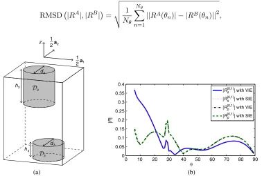
In the first test case the unit cell is defined by the lattice vectors a1 = ˆx400 nm, a2 = ˆy400 nm and it contains two dielectric cylinders embedded in a free-space background medium. The unit-cell configuration with the two cylinders and their dimensions is shown in Figure 3(a). The first cylindrical domainD2 is a dielectric withεr = 2.25, heighth2 = 225 nm, diameter d2 = 200 nm, and the center of the bottom surface is positioned at (−50,−50,50) nm. The second cylindrical domainD3 is a dielectric withεr = 3−3j, heighth3 = 100 nm, diameter d3 =d2= 200 nm, and the center of the bottom surface is positioned at (50,50,−275) nm.
We apply the SIE method, with and without tabulation of the QPGF and its gradient, to compute the reflection coefficients of the four diffraction orders that can be observed when the angle of incidence of an s-polarized plane-wave incident field of wavelength λ0 = 425 nm is scanned from θ = 0◦ to almost grazing incidence θ = 89◦ in steps of 1◦ while the azimuth angle is kept fixed at φ = 45◦. To validate the SIE implementation we have also computed the reflection coefficients with the VIE method presented in [31]. Detailed information on computing the reflection coefficients for the VIE method can be found in [32, Section 4]. To obtain accurate results with the VIE method we have used 63 modes in both the x and y direction and we have used 161 and 71 equidistant sample points in the z-direction for the cylindrical domains D2 and D3, respectively. In the SIE method we have used 304 and 320 triangular elements to discretize the boundaries of the cylindrical domains D2 and D3, respectively, which corresponds to a number of 912 and 960 unknowns connected to ∂D2 and ∂D3, respectively. In Figure 3(b) it can be seen that the magnitude of the co-polar and the cross-polar reflection coefficients for the diffraction order (0,1) computed with the SIE method without applying tabulation and with the VIE method show a good correspondence. Note that the diffraction order (0,1) is first observed at
θ= 6◦.
To compare computed reflection coefficients RA(θ) and RB(θ) we define the Root Mean Square Deviation (RMSD) between the reflection coefficients as follows
RMSD|RA|,|RB|= 1
Nθ Nθ
n=1
||RA(θn)| − |RB(θn)||2, (31)
1 2 1
2
0 10 20 30 40 50 60 70 80 90
0 0.05 0.1 0.15 0.2 0.25 0.3 0.35 0.4
|
R
|
|R(0,1)s | with VIE
|R(0,1)s | with SIE
|R(0,1)p | with VIE
|Rp(0,1)| with SIE
(a) (b)
θ
z
h
d
2
3 2
h 2
3 d
a2
a1
3
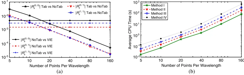
withNθ the number of angles for which the reflection coefficients are computed. The used definition of the RMSD implies that it only measures deviations between the magnitude of the reflection coefficients. We have computed the co-polar reflection coefficients for the diffraction orders (0,0), (0,1) and (1,1) using the SIE method with and without tabulation. More precisely, we have repeatedly applied the SIE method with tabulation using cubical grids of different edge length Δ = λ0/Nppwl withNppwl the number of points per wavelength.
In Figure 4(a) it is shown that the RMSD between the reflection coefficients computed using the SIE method with and without tabulation decreases quadratically with Nppwl. For each of the three co-polar reflection coefficients we have also indicated in the figure, with the horizontal lines, the RMSD between the reflection coefficients computed using the SIE method without tabulation and the VIE method. The figure shows that already for a cubical grid of edge length Δ =λ0/20, the RMSD between the reflection coefficients computed using the SIE method with and without tabulation is smaller than the RMSD between the reflection coefficients computed using the SIE method without tabulation and the VIE method.
In Figure 4(b) we show for the cubical grids of various edge lengths the required CPU time, averaged over the 90 angles, to build the look-up tables for the regularized QPGF and its gradient. In the figure, the measured average required CPU time is shown for four different methods of building the look-up tables. Method I is the proposed method that combines the computation of the regularized QPGF and its gradient for both the transverse vector rT −rT and for its opposite transverse vector rT −rT. Moreover, it uses the simplified expressions for the Ewald representation of the QPGF and its gradient fork2 >0 as presented in Appendix A. In Method II, the same tabulation strategy is applied but the average required CPU time has more than doubled because here we have used the Ewald representation of the QPGF and its gradient for generalk2 as is presented in Section 5. The average required CPU time has again almost doubled for Method III, where we still combine the computation of the regularized QPGF and its gradient but separately compute them for the transverse vector rT −rT and for its opposite transverse vector rT −rT. In Method IV, the regularized QPGF and its gradient have also been computed separately and as a consequence the average required CPU time has doubled once more. For all four methods the average required CPU time to build the tables increases cubically withNppwl. Note that building the interpolation tables is still cheap for the configuration under consideration but for unit cells that are larger in terms of wavelength this may no longer be the case, see for instance the analysis in [16, Section III-D]. In the latter case, a considerable gain in efficiency can be obtained if the strategy suggested in [5], in which only points of the interpolation table are filled if needed in a computation, is adopted.
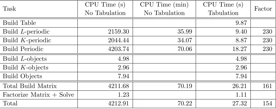
In Table 1, we compare the required CPU time, averaged over the 90 angles, for each of the subtasks in the SIE method in case we do or do not use tabulation of the QPGF and its gradient (with Δ =λ0/80). In the first column we have given the measured average CPU times for the SIE method
5 10 20 40 80 160
10 10 10 10 10
RMSD
Method I Method II Method III Method IV
(a) (b)
Number of Points Per Wavelength
5 10 20 40 80 160
Number of Points Per Wavelength
-1
-2
-3
-4
-5
10 10 10 10 10
10
-1
-2 3
2
1
0
Average CPU Time (s)
|R s(0, 0)| Tab vs NoTab |R | Tab vs NoTab s
(0, 1)
|R s | Tab vs NoTab
(1, 1)
|R s(0, 0)| NoTab vs VIE
|R s(0, 1)| NoTab vs VIE
|R s(1, 1)| NoTab vs VIE
without tabulation. In the second column the same average CPU times when larger than 60 seconds have been expressed in minutes. In the third column we have given the measured average CPU times for the SIE method with tabulation. In the fourth column we have listed the speed-up factor for each task when using tabulation. In the following, computation of the contribution to the MoM matrix by theL1 andK1 operators in (11) and (12) is respectively referred to as building theL-periodic operator and the K-periodic operator. Computation of the contribution to the MoM matrix by the L2 and L3 operators in (11) and (12) is referred to as building theL-object operators whereas computation of the contribution to the MoM matrix by theK2 and K3 operators in (11) and (12) is referred to as building the K-object operators. It is clear from the table that without tabulation the vast majority of the CPU time is spent on evaluating the QPGF and its gradient in the process of computing the periodic operators during the matrix build. By applying tabulation and interpolation we have managed to reduce the building time of both periodic operators by a factor of 230. The additional task of building the look-up tables is relatively cheap in terms of CPU time. Note that in practice the object operators only need to be computed once and can be reused for all angles. The average CPU time listed in the table for building the object operators is based on recomputing the object operators for all angles and can therefore be reduced by a factor of 90. This would further increase the total speed-up factor from 154 to 216. Since we have two objects with approximately the same number of RWGs on each of the objects the total number of RWG interactions needed to compute the two periodic operators is twice the total number of RWG interactions needed to compute the four object operators. Building the L-periodic operator however is less than twice as time-consuming as building the two L-object operators, which is an indication that computing the QPGF by interpolation may be even faster than computing the aperiodic Green function. Building the K-periodic operator however is more than twice as expensive as building the two K-object operators which may be caused by the large number of in-plane RWG interactions for which the contribution to theK-object operators is easily determined to be zero.
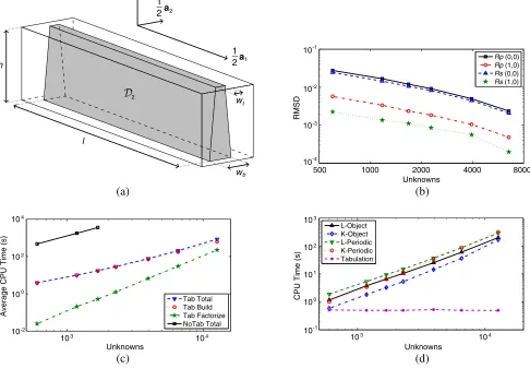
In the second test case the unit cell is defined by the lattice vectorsa1= ˆx500 nm,a2 = ˆy100 nm and it contains a copper truncated triangular prism embedded in a free-space background. The unit-cell configuration with the truncated triangular prism and its dimensions, length l = 460 nm, height
h = 120 nm, bottom width wb = 42 nm and top width wt = 18 nm is shown in Figure 5(a). The relative permittivity of the copper is taken to beεr=−17.3−1.78j which implies the structure exhibits plasmonic behavior.
We apply the SIE method, with tabulation of the QPGF and its gradient, to compute the reflection coefficients of the two diffraction orders that can be observed when the angle of incidence of a p-polarized plane wave incident field of wavelengthλ0 = 700 nm is scanned fromθ= 0◦ to almost grazing incidence θ = 89◦ in steps of 1◦ while the azimuth angle is kept fixed at φ = 45◦. The SIE computations are
Table 1. Comparison average CPU time SIE method with tabulation (80 points per wavelength) and without tabulation of the QPGF and its gradient.
Task CPU Time (s)
No Tabulation
CPU Time (min) No Tabulation
CPU Time (s)
Tabulation Factor
Build Table 9.87
BuildL-periodic 2159.30 35.99 9.40 230
BuildK-periodic 2044.44 34.07 8.87 230
Build Periodic 4203.74 70.06 18.27 230
BuildL-objects 4.98 4.98
BuildK-objects 2.96 2.96
Build Objects 7.94 7.94
Total Build Matrix 4211.68 70.19 26.21 161
Factorize Matrix + Solve 1.23 1.11
performed for seven MoM meshes of decreasing mesh size. All SIE computations with tabulation make use of a fine sampling grid of 100 points per wavelength. In Figure 5(b) we show that the RMSD in the co-polar and cross-polar reflection coefficients decrease linearly with the number of unknowns if we take the reflection coefficients computed with the finest mesh as the reference solution. In Figure 5(c) it is shown that the average required CPU time per angle for building the matrix and for factorizing the matrix respectively increases quadratically and cubically with the number of unknowns. However, for the first six meshes the cost of building the matrix still is dominant and the curve for the average required total CPU time per angle almost coincides with the curve for the matrix-build time. Also indicated in Figure 5(c) for the first three meshes is the average required total CPU time per angle in case the SIE method is applied without the use of tabulation and it can be seen that an improvement factor of more than 100 in computation time has been achieved by applying the tabulation. In Figure 5(d) the required CPU time for building the look-up tables and the L and K operators for the first angle is shown for each of the seven meshes. It is clear that with the use of tabulation the time required for evaluating the periodic operators and the object operators has become comparable. The time required for building theK-object operator is again the lowest, which may be explained by the many in-plane interactions that can easily be set to zero. Note that the object operators only have to be built for the first angle whereas the periodic operators have to be rebuilt for each new angle. Since we use the same look-up tables for each of the meshes the required CPU time to build these tables is constant and for this sub-wavelength cell it is very low. More results can be found in our ICEAA 2014 conference paper [33].
500 1000 2000 4000 8000
Unknowns
Rp (0,0) Rp (1,0) Rs (0,0) Rs (1,0)
Tab Total Tab Build Tab Factorize NoTab Total
L-Object K-Object L-Periodic K-Periodic Tabulation
(a) (b)
(c) (d)
1 2 1
2
z
h
a2
a1
l
w
t
b
w
10 10 10 10
RMSD
-1
-2
-3
-4
10 10 10 10 10
-1 3
2
1
0
CPU Time (s)
10 10 10
10-2 4
2
0
Average CPU Time (s)
Unknowns Unknowns
103 104 103 104
2
8. CONCLUSIONS
We have identified the SIE method to be very suitable for computation of electromagnetic fields scattered by 2D-periodic high-permittivity and plasmonic scatterers. Key to the feasibility of using the SIE method for 2D-periodic penetrable structures in an infinite homogeneous medium is the ability to efficiently evaluate the 2D-QPGF and its gradient. A successful strategy to accelerate computation of the 2D-QPGF and its gradient is to pre-compute and store the regularized 2D-QPGF and its gradient on a pre-defined interpolation grid so that the values needed to compute the numerical integrals in the method of moments (MoM) matrix can be obtained fast by using interpolation routines. We have presented an efficient technique to create the look-up tables for the QPGF and its gradient where we use to our advantage that it is very effective to simultaneously compute the QPGF and its gradient, and to simultaneously compute these values for the case in which the role of source and observation point are interchanged, thereby reducing the tabulation time by a factor of four. In the process of pre-computing the regularized 2D-QPGF and its gradient we apply the Ewald representation of the 2D-QPGF, which provides a robust method of evaluating the QPGF regardless of the loss properties of the medium and the position of observation and source point. Since there are dedicated algorithms to compute the scaled complex complementary error function, also referred to as the Faddeeva function, it is more efficient to use the Ewald representation of the 2D-QPGF in terms of the Faddeeva function. We have presented the expressions for the Ewald representation of the 2D-QPGF in terms of the Faddeeva function for both lossy and lossless medium parameters. Moreover, we have shown that the expression for the lossless case can be evaluated twice as fast as the expression for the lossy case. While the efficient tabulation technique in combination with interpolation can also be used to compute extracted terms in doubly periodic structures in layered media, the proposed method is validated here by computing the reflection coefficients for a plane-wave incident field impinging on an arbitrary number of mutually disjoint 2D-periodically repeated penetrable objects in a 3D homogeneous space. In two case studies we have shown that for unit cells that are not too large in terms of the wavelength the additional task of building the look-up tables is computationally cheap even when simple tri-linear interpolation is used. By using the tabulation technique in combination with the very fast tri-linear interpolation it has been shown that the time required for building the periodic operators has become comparable to the time required for building the object operators and as a result the total computation time is reduced with a factor of 100 or more.
APPENDIX A. EWALD REPRESENTATION QUASI PERIODIC GREEN FUNCTION IN TERMS OF THE FADDEEVA FUNCTION FOR K2 >0
In Section 5 we have shown that for general complexk2 we may express the Ewald representation of the QPGF and the Ewald representation of the gradient of the QPGF in terms of a scaled complementary error function, the Faddeeva function w(z). In the special case that k2 = ω2εμ > 0 we can use the properties of the Faddeeva function
w(−z) = 2e−z2−w(z), (A1)
w(z∗) = w(−z)∗, (A2)
where the star denotes complex conjugation, to simplify the Ewald representation of the QPGF and its gradient such that we only need one Faddeeva-function evaluation per term in the summation:
GspatialΛ,E,n = 1 4π
e−jkiT·an−(|Rn|E)2+(2kE)
2
|Rn| Re
w
j|Rn|E+ k 2E
, (A3)
∇GspatialΛ,E,n = 1 4π
e−jkiT·an−(|Rn|E)2+(2kE)2
|Rn|
−| 1
Rn|Re
w
j|Rn|E+ k 2E
+kIm
w
j|Rn|E+ k 2E
−√2E
π
Rn
|Rn|. (A4)
since a dedicated algorithm for real arguments is very efficient.
Propagating Modes ((γmz )2 =kTm·kmT −k2 <0):
GspectralΛ,E,m = 1 2A
e−jkmT·RT γzm
e−γzm(z−z)+e−
γm
z
2E
2
−((z−z)E)2
jIm
w
jγzm
2E +j(z−z
)E,(A5)
∇GspectralΛ,E,m = 1 2A
e−jkmT·RT γzm
(−jkmT −γzmˆz)e−γzm(z−z)
+kmT e−
γm
z
2E
2
−((z−z)E)2 Im
w
jγzm
2E +j(z−z
)E
+γzmˆze−
γm
z
2E
2
−((z−z)E)2 Re
w
jγzm
2E +j(z−z
)E . (A6)
Evanescent Modes((γzm)2=kTm·kmT −k2 >0):
GspectralΛ,E,m = 1 4A
e−jkmT·RT γzm
erfc
γzm
2E + (z−z
)Eeγm
z (z−z)
+erfc
γzm
2E −(z−z
)Ee−γm
z (z−z)
, (A7)
∇GspectralΛ,E,m = 1 4A
e−jkmT·RT γzm
(−jkmT +γzmˆz) erfc
γzm
2E + (z−z
)Eeγm
z (z−z)
+ (−jkmT −γzmˆz) erfc
γzm
2E −(z−z
)Ee−γm
z (z−z)
. (A8)
APPENDIX B. REFLECTION COEFFICIENTS
Letzmaxbe the maximumz-coordinate found in any of the objects. The reflected electromagnetic field for propagating modemforz > zmax is given by
Em,r(r) =
jωμ1
I− 1
k2 1
(km,r)km,r·
Fmr (J1)−jkm,r× Fmr(M1)
e−jkm,r·r
2γzmA , (B1)
Hm,r(r) =
jωε1
I− 1
k12
(km,r)km,r·
Fmr (M1) +jkm,r× Fmr(J1)
e−jkm,r·r
2γzmA , (B2)
whereI denotes the 3×3 identity matrix, km,r =kmT −jγzmˆz, and
Fr
m({J1,M1}) =−
∂D1
{J1,M1}(r)ejk m,r·r
dA. (B3)
We now follow [34, page 24] and introduce vectorial modal reflection coefficients Rm,e andRm,h in the following way:
Em,r(r) =Rm,ee−jkm,r·(r−zmaxˆz)
, Hm,r(r) =Y1Rm,he−jk
m,r·(r−zmaxˆz)
. (B4)
For each mode, we can further decompose the above plane-wave representation in terms of the parallel (p) and the perpendicular (s) polarization, which are different for each mode due to the different k -vectors. We define the unit vectors
ˆsm = k
m
T
|kmT |׈z, ˆs
m,⊥= ˆsm׈z=− kmT
|kmT |, (B5)
and define the reflection coefficients insand p polarization as
When the incident electric field at z = zmax has unit amplitude and zero phase, Rms and Rmp can be interpreted as the Fresnel reflection coefficients in s and p polarization, respectively. The final expressions for the reflection coefficients ins andp polarization are
Rms =
Z1Fmr (J1)·ˆsm+jγ
m
z
k1 F
r
m(M1)·ˆsm,⊥−|
kmT |
k1 F
r
m(M1)·ˆz
jk1e−γ m
z zmax
2γzmA , (B7)
Rmp =
Y1Fmr(M1)·ˆsm−jγ
m
z
k1 F
r
m(J1)·ˆsm,⊥+|
kmT |
k1 F
r
m(J1)·ˆz
jk1Z1e−γ m
z zmax
2γzmA . (B8)
REFERENCES
1. Kobidze, G., B. Shanker, and D. P. Nyquist, “Efficient integral-equation-based method for accurate analysis of scattering from periodically arranged nanostructures,”Physical Review E, Vol. 72, No. 5, 056702, Nov. 2005.
2. Sol´ıs, D. M., M. G. Ara´ujo, L. Landesa, S. Garc´ıa, J. M. Taboada, and F. Obelleiro, “MLFMA-MoM for solving the scattering of densely packed plasmonic nanoparticle assemblies,” IEEE Photonics Journal, Vol. 7, No. 3, 4800709, Jun. 2015.
3. Valerio, G., P. Baccarelli, S. Paulotto, F. Frezza, and A. Galli, “Regularization of mixed-potential layered-media Green’s functions for efficient interpolation procedures in planar periodic structures,”
IEEE Transactions on Antennas and Propagation, Vol. 57, No. 1, 122–134, Jan. 2009.
4. Celepcikay, F. T., D. R. Wilton, and D. R. Jackson, “Interpolation of 2D layered-medium periodic Green’s function,” Antennas and Propagation Society International Symposium (APSURSI), Toronto, Jul. 11–17, 2010.
5. Wilton, D. R., D. R. Jackson, and F. T. Celepcikay, “Efficient computation of periodic, layered media Green’s functions,”6th European Conference on Antennas and Propagation (EuCAP 2012), Prague, Mar. 26–30, 2012.
6. Celepcikay, F. T., “Efficient calculation of layered-medium periodic Green’s function,” PhD Thesis, University of Houston, Houston, Texas, Aug. 2010.
7. Yl¨a-Oijala, P., M. Taskinen, and J. Sarvas, “Surface integral equation method for general composite metallic and dielectric structures with junctions,” Progress In Electromagnetics Research, Vol. 52, 81–108, 2005.
8. Sol´ıs, D. M., J. M. Taboada, and F. Obelleiro, “Surface integral equation-method of moments with multiregion basis functions applied to plasmonics,” IEEE Transactions on Antennas and Propagation, Vol. 63, No. 5, 2141–2152, May 2015.
9. Dardenne, X. and C. Craeye, “Method of moments simulation of infinitely periodic structures combining metal with connected dielectric objects,” IEEE Transations on Antennas and Propagation, Vol. 56, No. 8, 2372–2380, Aug. 2008.
10. Gallinet, B., A. M. Kern, and O. J. F. Martin, “Accurate and versatile modeling of electromagnetic scattering on periodic nanostructures with a surface integral approach,” Journal of the Optical Society of America A, Optics and Image Science, Vol. 27, No. 10, 2261–2271, Oct. 2010.
11. Jorna, P., V. Lancelotti, and M. C. van Beurden, “Formulation and implementation of boundary integral equations for scattering by doubly periodic plasmonic and dielectric structures of infinite lateral extent,”International Conference on Electromagnetics in Advanced Applications (ICEAA), 1423–1426, Torino, Sep. 7–11, 2015.
12. Ewald, P. P., “Die berechnung optischer und elektrostatischer gitterpotentiale,”Annalen der Physik IV, Vol. 64, 253–287, 1921.
13. Jordan, K. E., G. R. Richter, and P. Sheng, “An efficient numerical evaluation of the Green’s function for the Helmholtz operator on periodic structures,” Journal of Computational Physics, Vol. 63, No. 1, 222–235, Mar. 1986.
14. Kambe, K., “Theory of electron diffraction by crystals, I. Green’s function and integral equation,”
15. Stevanovi´c, I., P. Crespo-Valero, K. Blagovi´c, F. Bongard, and J. R. Mosig, “Integral-equation analysis of 3-D metallic objects arranged in 2-D lattices using the Ewald transformation,” IEEE Transactions on Microwave Theory and Techniques, Vol. 54, No. 10, 3688–3697, Oct. 2006. 16. Li, S., D. A. van Orden, and V. Lomakin, “Fast periodic interpolation method for periodic unit
cell problems,” IEEE Transactions on Antennas and Propagation, Vol. 58, No. 12, 4005–4014, Dec. 2010.
17. Shi, Y. and C. H. Chan, “Multilevel Green’s function interpolation method for analysis of 3-D frequency selective structures using volume/surface integral equation,” Journal of the Optical Society of America A, Optics and Image Science, Vol. 27, No. 2, 308–318, 2010.
18. Poggio, A. J. and E. K. Miller, “Integral equation solutions of three dimensional scattering problems,” R. Mittra, editor, Computer Techniques for Electromagnetics, Pergamon Press, Elmsford, New York, 1973.
19. Chang, Y. and R. Harrington, “A surface formulation for characteristic modes of material bodies,”
IEEE Transactions on Antennas and Propagation, Vol. 25, No. 6, 789–795, Jun. 1977.
20. Wu, T. K. and L. L. Tsai, “Scattering from arbitrarily-shaped lossy dielectric bodies of revolution,”
Radio Science, Vol. 12, No. 5, 709–718, 1977.
21. Harrington, R. F., Field Computation by Moment Methods, Wiley-IEEE Press, 1993.
22. Rao, S. M., D. R. Wilton, and A. W. Glisson, “Electromagnetic scattering by surfaces of arbitrary shape,” IEEE Transactions on Antennas and Propagation, Vol. 30, No. 3, 409–418, May 1982. 23. Kustepeli, A. and A. Q. Martin, “On the splitting parameter in the Ewald method,” IEEE
Transactions on Microwave and Guided Wave Letters, Vol. 10, No. 5, 168–170, May 2000.
24. Oroskar, S., D. R. Jackson, and D. R. Wilton, “Efficient computation of the 2D periodic Green’s function using the Ewald method,” Journal of Computational Physics, Vol. 219, No. 2, 899–911, Dec. 2006.
25. Celepcikay, F. T., D. R. Wilton, D. R. Jackson, and F. Capolino, “Choosing splitting parameters and summation limits in the numerical evaluation of 1-D and 2-D periodic Green’s functions using the Ewald method,”Radio Science, Vol. 43, RS6S01, Sep. 2008.
26. Stevanovi´c, I. and J. R. Mosig, “Green’s function for planar structures in periodic skewed 2-D lattices using Ewald transformation,” 1st European Conference on Antennas and Propagation (EuCAP 2006), Nice, France, Nov. 6–10, 2006.
27. Abramowitz, M. and I. Stegun, Handbook of Mathematical Functions, Dover Publications, New York, 1965.
28. Gautschi, W., “Efficient computation of the complex error function,” SIAM J. Numer. Anal., Vol. 7, No. 1, 187–198, Mar. 1970.
29. Poppe, G. P. M. and C. M. J. Wijers, “More efficient computation of the complex error function,”
ACM Transactions on Mathematical Software, Vol. 16, No. 1, 38–46, Mar. 1990.
30. Zaghloul, M. R. and A. N. Ali, “Algorithm 916: Computing the Faddeyeva and Voigt functions,”
ACM Transactions on Mathematical Software, Vol. 38, No. 2, 1–22, Dec. 2011.
31. Van Beurden, M. C., “A spectral volume integral equation method for arbitrary bi-periodic gratings with explicit Fourier factorization,” Progress In Electromagnetics Research B, Vol. 36, 133–149, 2012.
32. Van Beurden, M. C., “Fast convergence with spectral volume integral equation for crossed block-shaped gratings with improved material interface conditions,” Journal of the Optical Society of America A, Vol. 28, No. 11, 2269–2278, 2011.
33. Jorna, P., V. Lancelotti, and M. C. van Beurden, “SIE approach to scattered field computation for 2D periodic diffraction gratings in 3D space consisting of high permittivity dielectric materials and plasmonic scatterers,”International Conference on Electromagnetics in Advanced Applications (ICEAA), 143–146, Aruba, Aug. 3–9, 2014.