Efficient Elimination of Multiple-Time-Around Detections
in Pulse-Doppler Radar Systems
Anatolii A. Kononov1, * and Jonggeon Kim2
Abstract—The paper introduces a new method for eliminating multiple-time-around detections in coherent pulsed radar systems with single constant pulse repetition frequency. The method includes the phase modulation of transmit pulses and corresponding phase demodulation at reception, which is matched to signals from the unambiguous range interval, and subsequent coherent integration followed
by successive CFAR processing in range and Doppler domains. The performance of the proposed
method is studied by means of statistical simulations. It is shown that the elimination performance can be essentially improved by optimizing the transmit phase modulation code. The optimization problem is formulated in terms of least-square fitting the power spectra of multiple-time-around target signals to a uniform power spectrum. Several optimum biphase codes are designed and used in the performance analysis. The analysis shows that the method can provide very high probability of elimination without noticeable degradation in the detection performance for targets from the unambiguous range interval.
1. INTRODUCTION
Coherent pulsed radars, or pulse-Doppler radar systems, are widely used in ground, airborne and shipborne deployments to provide target detection and tracking in the presence of clutter [1–5].
Pulse-Doppler radar measurements are inherently ambiguous in either range or velocity or both. This
ambiguity is caused by the periodical structure of pulse-Doppler waveforms both in time and frequency domains since typical pulse-Doppler waveform is a coherent pulse train with constant pulsewidth and pulse repetition frequency (PRF).
The nature of ambiguity is determined by the PRF mode and required intervals of unambiguous range and velocity measurements. High PRF mode is usually unambiguous in velocity but generally highly ambiguous in range; low PRF mode is unambiguous in range but generally highly ambiguous in velocity; and medium PRF mode is moderately ambiguous in both range and velocity. The ambiguous measurements result not only in uncertainty of the target’s true position or velocity but also in the folding of the clutter energy in the ambiguous dimension and in the creation of range or velocity blind zones. These complications are particularly of great concern in search and acquisition modes when there is little or no prior information on target coordinates.
Marine radars encounter especially severe complications due to ambiguous range measurements in the event of ducting propagation. One of the significant propagation phenomena for radar is atmospheric refraction [1, 3, 5], which refers to the property of the atmosphere to bend electromagnetic waves as they pass through the atmosphere. Ducting propagation, which is also known as an extreme form of superrefraction, occurs when the bending of radar waves causes the curvature radius of the waves to become less than or equal to the radius of curvature of the Earth. This bending results in trapping the electromagnetic energy transmitted by radar in a “parallel plate waveguide” near the earth surface [1].
Received 30 August 2016, Accepted 27 October 2016, Scheduled 14 November 2016
* Corresponding author: Anatolii A. Kononov (kaa50ua@gmail.com; akononov@onestx.com).
1 Research Center, STX Engine, 288 Guseong-ro, Giheung-gu, Yongin-si, Gyeonggi-do 446-915, Korea. 2 Defence Agency for
The meteorological conditions that may lead to the formation of superrefracting ducts are well known and described in the literature.
Spatially, ducts can occur either at ground level (surface ducts) or being elevated (elevated ducts). Surface ducts over the water surfaces, which are also called evaporation ducts, and elevated ducts can allow radar waveforms to propagate for very long distances beyond the geometric horizon. This fact can
be explained by that inside a duct the one-way power density attenuation in rangeR is approximated
as a function ofR−1 instead ofR−2 as in the case of free space propagation [1]. Ducts can dramatically impair or enhance radar coverage and range depending on whether each link terminal in the radar/target or radar/receiver pair is located in or out of the ducts.
Although the presence of the elevated and evaporation ducts can result in extended radar range, the consequences of their presence are negative rather than positive. The extended radar range means
that radar system can detect targets located at ranges R that are far beyond the unambiguous range
Rua given by
Rua=cTr/2 =c/(2Fr) (1)
whereTris the pulse repetition interval (PRI) and Fr = 1/Tr the PRF. In other words, in the presence
of ducting propagation the radar system can detect multiple-time-around targets, i.e., targets, which are located in the i-th trip range intervals [(i−1)Rua, iRua], where i = 2,3, . . .. According to real
observations reported in [7], ducting may increase the radar range by an order of magnitude with respect to that for normal propagation, e.g., for the area of Singapore Changi Airport, an increase from 33 km for normal propagation to 367 km for ducting propagation was observed. This is possible even in
low-PRF or medium-PRF radar systems because of very small propagation loss (R−1 attenuation law)
when both radar and targets at ambiguous ranges (R > Rua) are located in a duct.
Figure 1(a) illustrates a scenario with three targets that are within the radar antenna beamwidth at different ranges: Target 1 is located in the first trip (unambiguous) range interval at true rangeR1,
Target 2 and Target 3 are located in the 2-nd and 3-rd trip range intervals at true ranges R2 and R3,
respectively. Figure 1(b) shows ranges, at which the targets in Figure 1(a) may be detected by the radar if the radar and Targets 2 and 3 are located in a duct. Since Target 1 is located in the unambiguous range interval (R1 < Rua) this target is detected by the radar at the true rangeR1. Targets 2 and 3 are
0
Rua
R2a R1 R3a
Range Target 1
Target 2 Target 3
R2a= R2– Rua
R3a= R3–2Rua
(b) Coastline
Open sea
0
First trip range interval
Second trip range interval
Third trip range interval Target 1
Target 2 Target 3
Rua 2Rua 3Rua
Azimuth
R1 R2
R3
Radar
(a)
located in ambiguous range intervals (the 2-nd and 3-rd trip range intervals in this example), therefore these targets may be detected by the radar at the apparent rangesR2a=R2−RuaandR3a=R3−2Rua,
respectively.
The targets associated with multiple-time-around signals (shortly, thei-th trip targets), which can be detected by the radar in the case of ducting propagation, appear on radar display asfalse targets since they are misinterpreted as the 1-st trip targets at some false target positions, or in other words, they appear on the radar PPI as objects, which are not actually present at corresponding apparent ranges measured by the radar. Hence, the false targets confuse radar operators and waste the computational resources of radar tracker. Thus, the false targets are highly undesirable since they impede normal radar operations and create danger to the safety of navigation.
Another consequence of the extended radar ranges during ducting conditions is that precipitation and ground clutter from longer ranges folds into the unambiguous range-Doppler region. This folded clutter may result in the degradation of radar detection performance and increasing the false alarm rate unless constant false alarm rate (CFAR) processing is used by a radar signal processor.
Thus, to cope with the problem of false targets resulting from the presence of ducting propagation, a method is required, which would allow eliminating, with high probability, thei-th trip targets (i >1) and simultaneously maintaining acceptable detection probability for the 1-st trip targets at the specified false alarm rate, i.e., the method has to possess the CFAR property.
It is clear that eliminating the false targets caused by the ducting propagation is directly related to resolving range ambiguities of multiple-time-around targets. Once range ambiguity is resolved for targets detected by the radar, all the targets, for which the true ranges exceed the unambiguous range Rua, can be eliminated.
This paper addresses only the problem of resolution of the range ambiguity. All known methods that have been proposed to resolve the range ambiguity in pulsed radar systems can be divided into the following three basic classes.
First class of such methods is based on using multiple constant PRFs when the total coherent processing interval (CPI) is split into different sub-CPIs for transmitting pulse trains with different constant PRFs [1–6]. A conventional implementation of this method is based on using two pulse trains respectively having different constant PRFs, which are transmitted sequentially. This method has the following disadvantages:
- Increasing the number of PRFs implies that the dwell time (time-on-target) must be increased, hence, the total search or surveillance time increases, or the time (number of pulses) of each pulse train must be decreased, hence, the target signal-to-noise ratio (SNR) for each sub-CPI is reduced by the
factor 1/n (n stands for the number of PRFs) with respect to the value of the SNR that would be
obtained if a single constant PRF pulse train were used for the entire CPI frame.
- More PRFs are required than possible number of targets within a given CPI frame to avoid additional type of ambiguity called ghosting.
- For a detection to be declared for a given CPI frame, there must be detections on m out of n
(m-of-n criterion) of the multiple PRFs with typical requirements being 3-of-3 or 2-of-4 or 5-of-7, etc. Thus, multiple detections on partial PRFs with reduced SNR are required, and complex logic is needed to sort out these partial detections in order to declare a target detected on a given CPI frame.
The second class of methods for resolving the range ambiguity is based on phase coding, which can be implemented as a random phase coding, or in a deterministic manner when the phases of transmit pulses change according to a systematic (deterministic) phase code. Since these methods use a single constant PRF transmission they are free of the disadvantages of the multiple PRF methods.
US Patent No. 6,081,221 [8] describes a method for resolving range ambiguities in Doppler weather radars. For a single constant PRF transmission, the method consists of a special deterministic code for the phases of transmitted pulses as well as associated decoding and processing of return signals. The decoding process restores the coherency for the signals from the selected i-th trip interval (i= 1 or 2 is considered in [8]) while for the signals from other range intervals the coherency is not restored. Processing steps include a procedure of separating overlaid signals from the 1-st and 2-nd trip intervals and a procedure of estimating the spectral moments of separated signals. The method proposed in [8] does not possess the CFAR property.
which can eliminate targets associated with multiple-time-around signals or capable of removing range ambiguity of these multiple-time-around targets. The radar described in [9] employs the phase coding because it includes a device for changing the phases of transmitted pulses and it also includes devices for phase detecting received radar pulses and for integrating phase detected signals in a coherent manner. However, the radar according to US Patent 5,079,556 [9] does not maintain constant false alarm rate.
Inter-pulse coding based on binary sequences, which yield ideal (sidelobe free), low SNR loss, periodic cross-correlation with slightly mismatched reference sequence of the same length is suggested in [10] for mitigating range ambiguity in high PRF radars. It should be noted that ideal cross-correlation takes place only when the reference signal is exactly matched to a Doppler shift of the input signal. In the case of Doppler mismatch, the resulting cross-correlation is not sidelobe free which may seriously impair the mitigating of range ambiguity. Moreover, the method proposed in [10] does not include any processing means to ensure the CFAR property.
Techniques employing pulse-to-pulse diversity constitute the third basic class of methods for
resolving range ambiguities. These methods employ a set of N (N > 1) unique pulse modulation
codes that are selected based on orthogonality criteria or small level of cross-correlations. Each radar
transmitted pulse is coded with one of the N selected pulse codes. Once N coded pulses have been
transmitted, the process is repeated and another sequence ofN coded pulses is transmitted. The received
radar returns are simultaneously processed in N separate channels with each channel corresponding
to a distinct pulse code. Each channel is designed to suppress radar returns from all pulses except those containing the code corresponding to that channel. A nonlinear suppression technique (NLS) that employs this approach is considered in [11, 12]. This technique achieves the range ambiguity suppression through a combination of matched filtering and nonlinear “hole-punching” transformation designed to
remove undesired compressed pulse returns associated with mismatched codes. However, the NLS
method in [11, 12] does not include any processing means to ensure the CFAR property.
The present paper introduces a new method for efficient elimination of undesirable detections associated with multiple-time-around target returns in pulse-Doppler radars with single constant PRF. This new method uses the transmit phase modulation and corresponding phase demodulation at reception, which is matched to the first trip radar returns, combined with subsequent coherent integration and successive CFAR processing in range and Doppler domains. In detail, the proposed method includes phase modulation of pulses transmitted within each pulse repetition interval; restoring coherence of radar signals received from targets that are within the unambiguous range interval by means of phase demodulation; Doppler processing of all received radar signals to obtain their power spectra representation in Range/Doppler domain; target detection by means of CFAR processing in range (Range CFAR) using said representation in Range/Doppler domain; eliminating detections resulted from multiple-time-around target returns by means of CFAR processing in frequency domain (Doppler CFAR) for each detection reported by the Range CFAR.
The paper is organized as follows. Section 2 describes the proposed method using a block diagram of an exemplary pulse-Doppler radar system implementing the method. Section 3 discusses the choice of the transmit phase modulation codes and analyzes the transformation (after phase demodulation) of the power spectrum for the target signal associated with multiple-time-around returns with respect to that of the target signal from the unambiguous range interval. Section 4 studies the performances of the proposed method and addresses the problem of optimum design of the transmit phase modulation codes. Finally, Section 5 concludes our discussions.
2. DESCRIPTION OF THE METHOD
To describe the proposed method, we use block diagram (Figure 2) of an exemplary pulse-Doppler radar system, which performs phase coding and decoding (matched to the unambiguous range interval) as well as Doppler processing and CFAR detection that are realized by Radar Signal Processor (Figure 3). An implementation of successive Range/Doppler CFAR processing is illustrated in Figure 4, where an estimate of the average interference power around the cell under test (CUT) (m,n) in range and Doppler domain is computed as a function of the reference samples in range dimension ˆPr=fr(bsn),s∈Im, and
as a function of the reference samples in Doppler dimension ˆPd =fd(bmt), t ∈ Jm, respectively. The
Duplexer
Phase Code Generator Antenna
Upconverter Power
Amplifier LNA
Down Conversion/IF Amplifier (2 Stages) Frequency
Synthesizer
Master Oscillator
Waveform Generator Mixer
exp(jϕk)
ϕk
A/D Converter
Digital Down Converter
exp(-jϕk)
Radar Signal Processor
Radar Display
Upconverter
Pulse Compression
Phase coding
Phase decoding Doppler processing
CFAR detection
Figure 2. Block diagram of pulse-Doppler radar system implementing the proposed method.
of reference cells for the Range/Doppler CFAR. Figures 6(a) and 6(b) show the selection of reference
cells for the Doppler CFAR when the Doppler index n for the CUT n = 1 and n = N, respectively.
Block diagram in Figure 2 is suitable for any phase coding method, including arbitrary random coding. For instance, systematic Chu type codes or so called SZ (n/M) codes [8] can be used to implement the proposed method.
3. DESIGN OF PHASE MODULATION CODE
Systematic biphase (or binary) codes can be used in phase coding as a reasonable alternative to
multiphase Chu codes, SZ (n/M) codes and random codes. Biphase coding implies that the phases
of transmit pulses can take on one of the two possible values 0 (0◦) or π (180◦). Using biphase codes simplifies the radar implementation because no complex multiplications by exp(jϕk) and exp(−jϕk)
are required. It is clear that when a biphase code is used the phase coding and decoding is simply implemented by changing the sign of all the I and Q samples associated with the k-th transmit pulse
having the phase ϕk = π as well as for all the I and Q samples corresponding to the radar signals
received within the pulse repetition interval immediately following thek-th transmit pulse. No change of sign is required when the k-th transmit pulse has the phase ϕk = 0.
Figure 7 is a block diagram of the functioning of an exemplary version of a pulse-Doppler radar system when the proposed method is implemented using biphase coding. In Figure 7, the transmit waveform is represented by a set of real IF (intermediate frequency) samples, which are stored in waveform generator memory.
Further in this paper we consider phase coding based on systematic biphase codes. A reasonable approach to determining a suitable code is to use known family of codes. Thus, in the case of biphase coding binary Barker codes [1, 13], optimal periodic (OP) binary codes [14], minimum peak sidelobe (MPS) codes [1, 13] and maximum length sequences (MLS) [1, 13] can be used.
Windowed FFT
Range/Doppler CFAR
Data representing detections:
a set of Range/Doppler indices (mp, nq) and corresponding set of samples
P = the number of detected range bins Qp= the number of detected Doppler bins at the p-th range bin
Pulse Compression Output
To Radar Display
| . |2
A= [amn]
Nr-by-NRange/PRI complex data matrix representing PRI-to-PRI returns (N samples) for each of Nrrange bins (cells)
B= [bmn]
Nr-by-NRange/Doppler real data matrix representing Doppler profiles (N samples) for each of Nr range bins
p n m q p Q q P p b n
m pq
,..., 2 , 1 ; ,..., 2 , 1 ) ( ), , (
]
[
a
mnA
]
[
b
mnB
) ( q pn m b Squared-magnitude operation=
=
=
=
Figure 3. Block diagram of radar signal processor.
binary Barker codes are given. Examples of the OP codes are provided in [14] for 3 ≤ L ≤ 64. The
MPS codes through length 105 are provided in [1]. The MLS is a periodic binary sequence, whose pattern of ones and zeros does not repeat within a period L = 2n−1, n= 1,2, . . . [1, 13]. Any MLS is generated by means of a shift register employing feedback with binary coefficients and modulo 2 additions. The feedback coefficients that provide the maximum-length sequences are determined by an irreducible, primitive polynomial of degree n.
Hereinafter we assume that the length L of a code is equal to the maximum number of pulsesN
that can be processed by the radar signal processor during the coherent processing interval (CPI) frame that consists ofN successive pulse repetition intervals.
A sequence of phase states {0, π} corresponding to any given binary code is determined by the
conversions 0 → 0,1 → π. Taking into account the sign change for the data corresponding to the
transmitted pulses with phase π (see Figure 7) it is convenient to represent biphase codes using the complex exponential exp(jϕk). Thus, any biphase code consisting of phase states{0, π} yields a binary
sequence of elements{1,−1}, which can be represented as{+,−} for the sake of convenience.
Examples of the MPS and OP codes of length N = 16 are given in Table 1.
Table 1. Examples of binary codes of length 16.
MPS 0 1 1 0 1 0 0 0 0 1 1 1 0 1 1 1
[13, p. 108] + − − + − + + + + − − − + − − −
OP 1 1 1 1 1 0 1 0 1 1 0 0 0 1 0 0
[14, p. 134] − − − − − + − + − − + + + − + +
In Figure 2, the transmit pulses are periodically phase-shifted according to a periodic phase code sequence given byak= exp(jϕk),k= 1,2, . . .,N and the received echo samples are phase-demodulated,
i.e., are multiplied by the corresponding complex conjugate valuea∗k = exp(−jϕk) to restore the phases.
Collecting data representing detected cells: Range/Doppler indices (m, n) and
corresponding samples bmn. (m,n),bmn Collecting
]
[
b
mnB
Yes n = 1:N
r
mn P
b ˆ
m = 1:Nr
m sn
r
r f b s I
Pˆ ( ),
No
m mt
d
d f b t J
Pˆ ( ),
Yes
d
mn P
b ˆ No
End Estimating average interference power Pr
in range domain around the cell under test (m, n) according to a specified range CFAR method.
Imis a set of indices of reference samples
in range for the cell under test (m, n).
Estimating average interference power Pd
in Doppler domain around the cell under test (n, m) according to a specified Doppler CFAR method.
Jmis a set of indices of reference samples
in Doppler for the cell under test (m, n). Range CFAR thresholding
Doppler CFAR thresholding
=
=
α. >−
>− β. =
Figure 4. Successive range and Doppler CFAR processing.
code (TxPM code) and corresponding multiplication code sequence, respectively. When the biphase
coding technique is used the elements of the multiplication code sequence assumes only two possible values 1 or−1. Hence, in the case of biphase coding operations of complex multiplication are replaced with computationally simpler operations of sign inversion (see Figure 7). Consequently, after the phase demodulation the phase shift ϕk is fully compensated for the 1-st trip target signals but the 2-nd trip
target signals are phase modulated according to the sequence of phase differences ϕk−1−ϕk or to the
sequence of productsck =ak−1a∗k= exp[j(ϕk−1−ϕk)].
Generally, after the phase decoding the phasesψi,k of thei-th trip signal,i= 1,2, . . . are given by
ψ1,k = ϕk−ϕk; for the 1st trip signal
ψ2,k = ϕk−1−ϕk; for the 2-nd trip signal
. . .
ψi,k = ϕk−i+1−ϕk; for thei-th trip signal
Thus, the first trip signals are made coherent while the signals from the second-, third- and other higher-order trips, i.e., all the i-th trip signals, i > 1, are phase modulated according to the sequence of phases ψi,k or to the corresponding sequence of productsci,k=ak−i+1a∗k= exp[j(ϕk−i+1−ϕk)].
When a systematic biphase code is used, the phase modulation for the i-th trip signal after the phase demodulation is easy to represent using the corresponding sequence ci,k = ak−i+1ak, which
elements assume only two possible values 1 or −1. To determine thei-th phase modulation sequence
ci,k,k= 1,2, . . .,N, it is convenient to consider anN-by-N matrixAof all cyclic shifts of a row-vector
G
G G
G
R
ange
b
ins
CUT (cell under test)
m
n
Doppler bins
G
Reference cell in range (for Range CFAR)
Guard cell Reference cell in Doppler
(for Doppler CFAR) Fragment of matrix B
around the cell under test (m,n)
Figure 5. Selection of reference cells for Range and Doppler CFAR.
Doppler bins
1 2 … N
G G m
Range bins
Doppler bins
1 2 … N
G G G
Range bins m
(a) (b)
Figure 6. Selection of reference cells for Doppler CFAR whenn= 1 andn=N. (a) Doppler bin index nfor the CUT is equal to 1. (b) Doppler bin index nfor the CUT is equal toN.
matrix A is the vector a. Table 2 shows an example of the 16-by-16 matrix A when the OP code
from Table 1 is used as a periodic TxPM code. From the matrix A, the i-th trip signal modulation
sequence ci,k , i= 1,2, . . .,N is computed as an element-wise product of the first row elements by the
corresponding i-th row elements. Table 3 shows the matrix C, in which the i-th row represents the
phase modulation sequence ci,k computed using the corresponding rows of the matrix A. In Tables 2
and 3 the symbol “−” stands for −1 and the symbol “+” stands for 1.
Duplexer
Biphase Code Generator Antenna
Upconverter Power
Amplifier LNA
Down Conversion/IF Amplifier (2 Stages) Frequency
Synthesizer
Master Oscillator
Waveform Generator Real IF Samples
k
A/D Converter
Digital Down Converter
Sign Invertor Radar Signal
Processor
Radar Display
Upconverter
Pulse Compression Sign
Invertor D/A Converter
ϕ
Figure 7. Block diagram of pulse-Doppler radar system in the case of biphase coding.
Table 2. Matrix A— Cyclic shifts of multiplication code.
1 2 3 4 5 6 7 8 9 10 11 12 13 14 15 16
1 − − − − − + − + − − + + + − + +
2 + − − − − − + − + − − + + + − +
3 + + − − − − − + − + − − + + + −
4 − + + − − − − − + − + − − + + +
5 + − + + − − − − − + − + − − + +
6 + + − + + − − − − − + − + − − +
7 + + + − + + − − − − − + − + − −
8 + + + + − + + − − − − − + − + −
9 − + + + + − + + − − − − − + − +
10 + − + + + + − + + − − − − − + −
11 − + − + + + + − + + − − − − − +
12 + − + − + + + + − + + − − − − −
13 − + − + − + + + + − + + − − − −
14 − − + − + − + + + + − + + − − −
15 − − − + − + − + + + + − + + − −
16 − − − − + − + − + + + + − + + −
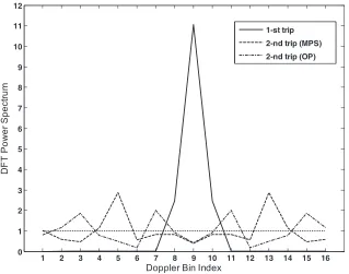
introduced at the transmission is fully compensated after the phase demodulation. Figure 8 compares the DFT power spectrum of the 1-st trip signal and that of the 2-nd trip signal for the TxPM codes of
1 2 3 4 5 6 7 8 9 10 11 12 13 14 15 16 0
1 2 3 4 5 6 7 8 9 10 11 12
D
FT P
o
w
e
r S
pect
ru
m
Doppler Bin Index
1-st trip
2-nd trip (MPS)
2-nd trip (OP)
Figure 8. Power spectra of the 1-st and the 2-nd trip signals for TxPM codes from Table 1.
Table 3. Matrix C — Phase modulation sequences.
1 2 3 4 5 6 7 8 9 10 11 12 13 14 15 16
1 + + + + + + + + + + + + + + + +
2 − + + + + − − − − + − + + − − +
3 − − + + + − + + + − − − + − + −
4 + − − + + − + − − + + − − − + +
5 − + − − + − + − + − − + − + + +
6 − − + − − − + − + + + − + + − +
7 − − − + − + + − + + − + − − − −
8 + − − − + + − − + + − − + + + −
9 + + − − − − − + + + − − − − − +
10 − + + − − + + + − + − − − + + −
11 + − + + − + − − − − − − − + − +
12 − + − + + + − + + − + − − + − −
13 + − + − + − − + − + + + − + − −
14 + + − + − − + + − − − + + + − −
15 + + + − + + + − − − + − + − − −
16 + + + + − − − − + − + + − − + −
The vector S= [S1, S2, . . . , SN] representing the DFT power spectrum of a signalu specified by a
vector of samples u= [u1, u2, . . . , uN] is computed as
S =|U|2, U =F F T[u] (2)
where U = [U1, U2, . . . , UN] is the vector of complex DFT samples, and vector u is normalized so that
which are summarized in Table 4. The Fast Fourier Transform (FFT) is implemented according to the following Matlab notation fftshift (fft (u,N )).
The unit-norm vector u corresponding to thei-th trip signal is computed according to
u=ci◦gant◦w◦uo
u=u/u
ci = [ci,1, ci,2, . . . , ci,N], ci,k∈ {−1,1}
uo = [1,exp(j2πy),exp(j2π2y), . . . ,exp(j2π(N −1)y)]
(3)
where ci is computed as the i-th row of the matrix C for the specified cyclic shift of a given TxPM
code; the vector gant represents the amplitude modulation of received signals by antenna pattern (see
Table 4); w is the vector of weighting coefficients (see Table 4); the symbol ◦ stands for the element wise product of vectors; y = fd/Fr is the normalized (unitless) Doppler frequency with fd being the
Doppler frequency in Hertz and Fr being the pulse repetition frequency in Hertz.
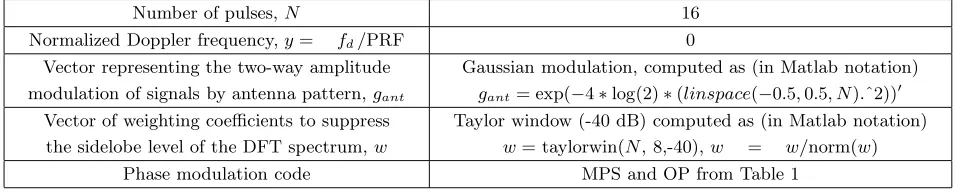
Table 4. Inputs used in computing power spectra.
Number of pulses,N 16
Normalized Doppler frequency,y= fd/PRF 0
Vector representing the two-way amplitude modulation of signals by antenna pattern,gant
Gaussian modulation, computed as (in Matlab notation) gant= exp(−4∗log(2)∗(linspace(−0.5,0.5, N).ˆ2))
Vector of weighting coefficients to suppress the sidelobe level of the DFT spectrum,w
Taylor window (-40 dB) computed as (in Matlab notation) w= taylorwin(N, 8,-40),w = w/norm(w) Phase modulation code MPS and OP from Table 1
As can be seen in Figure 8, the power spectrum of the 1-st trip signal is concentrated around zero Doppler frequency (around Doppler bin indexd=N/2 + 1 = 9 since the relationship betweendand the normalized Doppler frequency is given by y = (d−9)/16, d= 1,2, . . . ,16), while the power spectrum of the 2-nd trip signal for the OP code and that for the MPS code spreads over the entire Doppler axis. The power spectrum of signals associated with other higher-order trips exhibits similar behavior.
The distinction between the spectrum shape of the 1-st trip and the 2-nd (as well as other higher-order trips) suggests using CFAR processing in Doppler domain (Doppler CFAR) in addition to CFAR in range domain (Range CFAR) for eliminating the higher order trip signals without serious detrimental effect on the detection of the 1-st trip signal. The Range CFAR and Doppler CFAR differ from each other in a manner of taking the reference samples. For the Range CFAR the reference samples are selected from the samples surrounding a given cell under test (CUT) in range dimension while for the Doppler CFAR the reference samples are selected from the samples surrounding the CUT along Doppler dimension. Figure 5, Figures 6(a) and (b) show how the reference samples for the Range CFAR and Doppler CFAR are selected from the CUT surrounding samples. The physical rationale for combining Range/Doppler CFAR processing is discussed below.
conditions being equal. Thus, using the transmit phase modulation and phase demodulation, which is matched to the 1-st trip signal, in combination with Range/Doppler CFAR provides the possibility to efficiently eliminate the higher-order trip target without noticeable degradation in the detection probability for the 1-st trip target.
4. PERFORMANCE ANALYSIS
To characterize the overall detection performance for thei-th trip target,i= 1,2, . . ., we use the concept of overall detection probability, which is the probability that at least one sample Sk from the target’s
Doppler profileS = [S1, S2, . . . , SN] is detected after combined Range/Doppler CFAR. It should also be
noted that for the higher-order trip targets (i.e., when i >1) the term target elimination performance
is also relevant because the lower the detection probability for this kind of targets, the higher the target elimination probability, i.e., the probability that the target is not detected, or in other words, it is eliminated. If the i-th trip target (i > 1) overall detection probability is PODi then the corresponding elimination probabilityPEi is given byPEi = 1−PODi .
To estimate the efficiency of the proposed method, we compute the overall detection performance for the 1-st and higher-order trip targets using statistical simulation with 106 independent Monte-Carlo trials. The computations are carried out under assumption that the radar receiver noise obeys a zero-mean Gaussian distribution and the RCS fluctuations for the 1-st and thei-th trip targets (i >1) obey
the Swerling 1 model. Both I and Qsamples of noise are simulated as independent Gaussian random
values with unit variance σ2= 1.
The 1-st trip target signal is simulated according to
u(1) =2P1t·(gant◦w◦uo) (4)
where the 1-st trip target power P1t is generated as an exponential random variable with mean
¯
P1t = SN R1tPn, where SN R1t is the signal-to-noise ratio for the 1-st trip target and Pn = σ2 the
receiver noise power.
Thei-th trip (i= 2,3, . . .) target signal is simulated according to
u(i)=2Pit·(ci◦gant◦w◦uo)
ci = [ci,1, ci,2, . . . , ci,N], ci,k∈ {−1,1}
(5)
where the i-th trip target power Pit is also generated as an exponential random variable with mean
¯
Pit =SN RitPn where the SN Rit is the signal-to-noise ratio for the i-th trip target. The vectors gant
and w and other parameters, which we use in computing the detection performance, are specified in
Table 4.
In Equation (5), it is assumed that a sequence of pulses for thei-th trip target captured within any CPI frame contains Ncpi =N pulses (the case Ncpi < N is considered later). It is also assumed that
radar antenna is continuously rotating in azimuth at a constant angular velocity and the sequence ofN transmitted phases associated with the i-th trip target signal is simulated as a random vector, which
possible outcomes are all the N cyclic shifts of a given periodic TxPM code. Each of these outcomes
is assigned the probability 1/N. Therefore, the vectorci in Equation (5) is also simulated as a random
vector, which allN possible outcomes are equally probable. It is clear that all the possible outcomes for ci are determined by the corresponding cyclic shifts of a given TxPM code. This model for the sequence
of N transmitted phases takes into account the random location of targets in azimuth. In the present paper the performance analysis is carried out using this model.
In our performance study, the Range and Doppler CFAR are implemented according to the
conventional cell averaging (CA) CFAR algorithm. For the range CFAR, the number of reference
samples M = 24, the design false alarm probability Pf aRng = 10−6 and the corresponding threshold
multiplier α = 0.7782794. The parameters of the CA CFAR algorithm for the Doppler CFAR are
summarized in Table 5, where Pf aDop stands for the design probability of false alarm and β is the
corresponding threshold multiplier. The parameters α andβ are computed from the same equation [1,
p. 600], which is written below in terms ofβ
β=Pf a−1/M−1 (6)
Table 5. Parameters of CA CFAR algorithm for Doppler CFAR.
M = 13 Pf aDop 10
−1.0 10−1.5 10−2.0 10−2.5 10−3.0 10−3.5 10−4.0
β 0.1937766 0.3043214 0.4251027 0.5570684 0.7012543 0.8587919 1.0309176
4.1. Known Biphase Codes for Phase Modulation
This subsection analyzes the performance of the proposed method for the random phase modulation and that for the systematic biphase modulation when the radar uses known biphase codes. In the case of random phase modulation, the phases are generated as independent random values uniformly distributed on [0 2π]. The detection probability of interest is computed versus the design false alarm probability Pf aDop assuming equal SNR for the 1-st and 2-nd trip targets, i.e.,SN R1t=SN R2t= 10 dB.
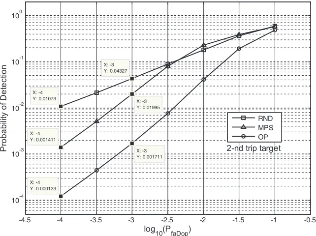
Figure 9 compares the estimated overall detection probabilityPDO2 for the 2-nd trip target in the case of random phase modulation (curve marked by RND) and deterministic biphase modulation with the MPS and OP codes from Table 1. Figure 10 shows the estimated detection probability for the 1-st trip target after the Range CFAR PDRng1 and the overall probability of detection PDO1 . The detection performance for the 1-st trip target does not depend on the phase modulation code because the phase modulation introduced into transmit pulses is completely removed from the 1-st trip target signal after the phase demodulation stage. Figure 11 plots the loss in the probability of detection L1P D (in percent) for the 1-st trip target, where the lossL1P D is computed as
L1P D = 100·(PDRng1 −PDO1 )/PDRng1 (7)
The estimated value of loss L1P D at Pf aDop = 10−1 is equal to zero. In order to present this zero-loss
point in logarithmic scale of Figure 11 we use the value of loss at point Pf aDop = 10−1.5.
From Figure 9, it is seen that the biphase modulation with the OP code outperforms that with the MPS code, e.g., at Pf aDop = 10−3, the estimated overall detection probability for the 2-nd trip target
in the case of the OP code isPDO2 = 1.71×10⁻³ which is noticeably less than PDO2 = 19.95×10⁻³ for the MPS code. As shown in Figure 9, the 2-nd trip target elimination performance in the case of the
-4.5 -4 -3.5 -3 -2.5 -2 -1.5 -1 -0.5
10-4 10-3 10-2 10-1 100
X: -3 Y: 0.04327
log10(PfaDop)
Pr
obabi
lit
y
of
Det
e
c
ti
o
n
X: -4 Y: 0.000123 X: -4 Y: 0.001411
X: -4
Y: 0.01073 X: -3 Y: 0.01995
X: -3 Y: 0.001711
RND MPS OP
2-nd trip target
-4.5 -4 -3.5 -3 -2.5 -2 -1.5 -1 -0.5 0.75
0.8 0.85 0.9
X: -4 Y: 0.8248
log
10(PfaDop)
Pr
o
babi
lit
y
o
f
D
e
te
c
ti
o
n
1-st trip target
X: -4 Y: 0.8187
Overall Range CFAR
Figure 10. Comparison of overall detection probability and detection probability after Range CFAR for the 1-st trip target.
-4.5 -4 -3.5 -3 -2.5 -2 -1.5 -1 -0.5
10-4 10-3 10-2 10-1 100
X: -4 Y: 0.7538
log10(PfaDop)
Loss (
%
)
X: -3.5 Y: 0.2827
X: -3 Y: 0.08138
X: -2.5 Y: 0.01417
X: -2 Y: 0.001212
X: -1.5 Y: 0.0001212 1-st trip target
Figure 11. Loss in detection probability for the 1-st trip target.
random phase modulation is essentially worse than that of the deterministic biphase modulation. Thus, we do not suggest random phase modulation for the implementation of the proposed method.
Analyzing the plots in Figure 10 and Figure 11 yields that the price paid for achieving reliable elimination performance for the 2-nd trip target is negligible. Indeed, even atPf aDop = 10−4 the loss in
the detection probability for the 1-st trip target L1
P D = 0.754% while the 2-nd trip target elimination
performance is excellent. Indeed, from Figure 9, the estimated value ofP2
DO forPf aDop = 10−4 is at a
4.2. Optimum Biphase Codes for Phase Modulation
One can draw two important inferences from the results presented in Figures 9 and 10. First, it is clear that adjusting the threshold multiplier in the Doppler CFAR allows achieving efficient target elimination for the 2-nd trip target without noticeable degradation in the detection performance for the 1-st trip target. Second, comparing the graphs plotted in Figure 9 for the OP and MPS codes yields that in the case of deterministic biphase modulation the choice of modulation code can be governed by the purpose of achieving the best performance. Generally, this means that the TxPM code can be optimized using the minimum of the overall detection probability for thei-th trip (i >1) target as an optimality criterion. Unfortunately, this optimization problem is very complex and we did not find any closed form solution for it.
However, the following approach to the aforesaid optimization problem can be suggested to find approximate solution. This approach is based on the following physical considerations. From Figure 9 and Figure 10, it is seen that the overall detection probability for the 1-st trip target is significantly higher than that for the 2-nd trip target. The physical reason for this is suggested by comparing the Doppler profiles (i.e., power spectra) for the signals corresponding to the 1-st and 2-nd trip targets: examples of the Doppler profiles for the 1-st and 2-nd trip targets are given in Figure 8. As one can see, a significant portion of the power for the 1-st trip target signal is concentrated in one dominant sample of its Doppler profile while the other samples of the profile are significantly lower than the dominant one. The dominant sample is significantly higher than the adaptive threshold for both the Range CFAR and Doppler CFAR, because the adaptive threshold is computed from the low level samples surrounding the dominant sample. Due to this the overall probability of detection for the 1-st trip target can be maintained at a certain high level depending on how large theSNR1tis. In contrast to the 1-st trip target,
the Doppler profile for the 2-nd trip target is spread over the entire Doppler axis with no significant difference between the samples. This results in decreasing the probability of detection for the 2-nd trip target after the Range CFAR processing and especially after the Doppler CFAR. Indeed, the adaptive threshold in the Doppler CFAR is computed from the samples, which are comparable in magnitude. Hence, when the Doppler CFAR thresholding is performed for each sample in the corresponding Doppler profile the probability of exceeding the adaptive threshold becomes essentially lower than that for the dominant sample in the Doppler profile associated with the 1-st trip target signal. Thus, the overall detection probability for the 2-nd trip target becomes essentially lower than that for the 1-st trip target. Based on the discussion above, one can assume that the overall detection probability for the 2-nd trip target is expected to be close to a certain minimum when the TxPM code provides such a power spectrum for the 2-nd trip target signal, which all spectral samples are as close to some constant level as possible, or, in other words, which provides the best fit to a uniform spectrum. To quantify the goodness of fit we use the standard squared Euclidean distance D, which is given by
D=
N
k=1
(Sk−So)2 (8)
whereSkis thek-th spectral sample of the corresponding power spectrum andSothe specified constant
level, i.e., the magnitude of the uniform spectrum.
According to the Parseval’s theorem the relationship between the signal vector u and its DFT
power spectrumS, see Equation (2), is given by
N
k=1
|uk|2=
1 N
N
k=1
|Uk|2 (9)
The right-hand side in Equation (9) represents the mean value of the power spectrum, and the left-hand side is the norm u of the vector u. When the vector u is normalized, i.e., u = 1, the mean value of the power spectrum is also equal to 1. Therefore, it is reasonable to set So = 1 in Equation (8),
because for any unity-norm vector u the mean value of the corresponding power spectrum is equal to
unity regardless of the TxPM code.
optimal under the criterion of minimum overall detection probability. However, based on the above
physical considerations one may expect that a TxPM code, which is optimal under the minimum D
criterion, should provide the overall detection probability that is close to a minimum provided by the code which is optimal under the criterion of minimum overall detection probability for the i-th trip targets (i >1).
Since the norm of the signal vector for any i-th trip target does not depend on thei-th trip phase
modulation sequence ci, in optimizing the TxPM code we use the unity-norm signal vector given by
Equation (2), where the vector ci is determined by the corresponding TxPM code that changes during
optimization procedure.
Strictly speaking, the minimumD criterion cannot be directly used in optimizing the TxPM code
when the sequence of N transmitted phases associated with the i-th trip target signal is modeled as a random vector, which possible outcomes are all theN cyclic shifts of a given periodic TxPM code. One of the possible optimality criteria that can be used with this model is the so-called “minimax criterion”. The procedure based on the minimax criterion that we use in optimizing the TxPM codes is explained below.
Table 6 summarizes all the TxPM biphase codes of lengthN = 16 that are globally optimum under
the minimax distance criterion for the 2-nd trip target. The codes are found by using the exhaustive search algorithm under the conditionNcpi=N. In the process of searching all 2N−1 possible non-zero
binary codes of length N are analyzed in turn. For the p-th analyzed code all the N distances Dq,
q = 1,2, . . . , N corresponding to the N possible cyclic shifts of the analyzed code are computed from Equation (8) and the maximum distance Dmax(p) = max{Dq, q = 1,2, . . . , N}, p = 1,2, . . . ,2N −1
and the corresponding cyclic shift are fixed. Then, the minimax distance Dmin max is determined as
Dmin max= min{Dmax(p), p= 1,2, . . . , 2N −1}and all the fixed cyclic shifts that meet the optimality
condition Dmax(p) =Dmin max are selected with no repetition.
Table 6. Optimum TxPM biphase codes of length 16 for the 2-nd trip target.
0 0 0 0 0 1 1 1 1 0 0 1 0 1 1 1 0 0 1 0 0 0 0 1 1 0 1 0 0 1 0 1 0 1 0 1 0 0 1 0 1 1 0 0 0 0 1 0 0 1 1 1 0 1 0 0 1 1 1 1 0 0 0 0 1 0 0 0 1 0 1 1 0 0 0 0 1 1 1 1 1 0 1 0 1 1 0 1 0 0 1 1 1 1 0 1 1 1 0 1 1 1 1 0 0 1 0 1 1 0 1 0 1 1 1 1 1 0 0 0 0 1 1 0 1 0 0 0
Following the circular shift theorem for the DFT, the power spectra corresponding to all the cyclic shifts of a given sequence of samplesx1, x2, . . . , xN are identical. However, in our optimization procedure
the distancesDq,q= 1,2, . . . , Nare computed for all cyclic shifts of a given TxPM code. This is because
the power spectra of thei-th trip target signals associated with these cyclic shifts are not identical: due to amplitude modulation of the received signal by the antenna pattern and/or amplitude weighting before the Doppler processing the i-th trip signals corresponding to different cyclic shifts of a given TxPM code are not the cyclic shifts of each other.
It is interesting to compare the minimax distance for the OP code from Table 1 and that for the
optimum TxPM codes from Table 6. The computations give Dmin max = 18.085 for the OP code and
Dmin max= 7.116 for all the optimum TxPM codes in Table 6. Hence, one can expect that the optimum
codes from Table 6 improve the 2-nd target elimination performance with respect to the OP code from Table 1.
-4.5 -4 -3.5 -3 -2.5 -2 -1.5 -1 -0.5 10-5
10-4 10-3 10-2 10-1 100
X: -1 Y: 0.3469
log10(PfaDop)
P
robab
ilit
y
o
f D
e
te
c
tio
n
X: -2 Y: 0.01131
X: -1 Y: 0.48
X: -2 Y: 0.04097
X: -3 Y: 0.000515 X: -3
Y: 0.001718
X: -4 Y: 0.000115
X: -4 Y: 4e-005
OP code (Table 1)
Opt code (Table 6) 2-nd trip target
Figure 12. Comparison of the 2-nd trip target elimination performance for the optimum biphase code from Table 6 (1-st row) and that for the OP code from Table 1.
-4.5 -4 -3.5 -3 -2.5 -2 -1.5 -1 -0.5
10-4 10-3 10-2 10-1 100
X: -2 Y: 0.1175
log10(PfaDop)
P
robabi
lity
o
f
D
e
te
c
ti
o
n
X: -3 Y: 0.005798
X: -2 Y: 0.05984
X: -3 Y: 0.002653
X: -4 Y: 0.000411
X: -4 Y: 0.000167
X: -1 Y: 0.5328 Opt code (Table 6)
OP code (Table 1) 3-rd trip target
Figure 13. Comparison of the 3-rd trip target elimination performance for the optimum biphase code from Table 6 (1-st row) and that for the OP code from Table 1.
at Pf aDop = 10−2 the gain in the overall probability detection is about 3.62 (0.04097/0.01131) and
gradually decreases to about 2.87 at pointPf aDop = 10−4. The Monte-Carlo simulations show that the
overall detection probability exhibits similar behavior for all the codes in Table 6.
terms of the 2-nd target elimination performance, their performance becomes worse than that for the OP code in the case of the 3-rd trip target as illustrated in Figure 13. To overcome this disadvantage, we construct an integrated goodness of fit measure DM C by averaging the goodness of fit measures for
the 2-nd and the 3-rd trip targets
DM C= 0.5 (D2+D3) (10)
whereD2 and D3 are computed from Equation (8) for the 2-nd and 3-rd trip targets, respectively.
Table 7 summarizes all the TxPM biphase codes of lengthN = 16 that are globally optimal under
the minimax DM C criterion for the 2-nd and 3-rd trip targets. The codes in Table 7 are found under
the condition Ncp =N by means of the same optimization procedure that is used for optimizing the
TxPM codes given in Table 6.
Table 7. Optimum biphase codes of length 16 for the 2-nd and 3-rd trip target.
0 0 0 0 1 0 0 1 0 1 0 1 1 1 0 0 0 1 0 1 1 1 0 0 0 0 0 0 1 0 0 1 1 0 1 0 0 0 1 1 1 1 1 1 0 1 1 0 1 1 1 1 0 1 1 0 1 0 1 0 0 0 1 1
Figure 14 compares the 2-nd, 3-rd and 4-th trip target elimination performances of the proposed method for the optimum TxPM code from the 1-st row of Table 7 and that for the OP code from Table 1. From Figure 14, it is seen that the optimum code from Table 7 maintains good false targets elimination ability and outperforms the OP code in all cases in question. It should also be noted that the gain in performance for the optimum code from Table 7 is larger for the higher-order trip targets. The Monte-Carlo simulations show that this effect takes place for all the TxPM codes in Table 7.
Figure 15 shows the effect of the signal-to-noise ratio (SNR) on the 2-nd trip target elimination performance in the case of the optimum TxPM code from Table 7 (1-st row). It is evident from this figure
-4.5 -4 -3.5 -3 -2.5 -2 -1.5 -1 -0.5
10-5 10-4 10-3 10-2 10-1 100
log10(PfaDop)
Pr
obab
ilit
y
o
f D
e
te
c
ti
o
n
2-nd trip target: OP code (Table 1) 2-nd trip target: Opt code (Table 7) 3-rd trip target: OP code (Table 1) 3-rd trip target: Opt code (Table 7) 4-th trip target: OP code (Table 1) 4-th trip target: Opt code (Table 7)
-4.5 -4 -3.5 -3 -2.5 -2 -1.5 -1 -0.5 10-6
10-5 10-4 10-3 10-2 10-1 100
log
10(PfaDop)
Pr
obab
ilit
y
o
f D
e
te
c
ti
o
n
SNR = 5 dB SNR = 10 dB SNR = 15 dB
Opt code (Table 7) 2-nd trip target
Figure 15. Elimination performance for the 2-nd trip target at different SNR.
Time Current CPI frame (8 PRIs)
h2= T{c2, 7 at leading part} = [c2,2 c2,3 c2,4 c2,5 c2,6 c2,7 c2,8 0]
Time Current CPI frame (8 PRIs)
h2= T{c2, 6 at trailing part} = [0 0 c2,1 c2,2 c2,3 c2,4 c2,5 c2,6]
Time PRI Current CPI frame (8 PRIs)
1-st trip target returns 2-nd trip target returns Transmitted pulse
h2= T{c2, 8} = [c2,1 c2,2 c2,3 c2,4 c2,5 c2,6 c2,7 c2,8]
(a) Ncpi= 8
(b)Ncpi= 7
(c) Ncpi= 6
Figure 16. Sequences ofNcpi pulses for the 2-nd trip target captured over current CPI frame.
that increasing the SNR results in noticeable improving the 2-nd trip target elimination performance forPf aDop ≤10−2.5.
So far the i-th trip target elimination performance of the proposed method is analyzed under the conditionNcpi=N, i.e., when the number of pulses actually captured over a given CPI frame is equal to
In this case thei-th trip (i= 2,3, . . .) target signal is simulated as
u(i)=2Pit·(hi◦gant◦w◦uo)
hi =T{ci, Ncpi}
ci = [ci,1, ci,2, . . . , ci,N], ci,k∈ {−1,1}
(11)
where Pit is simulated as an exponentially distributed random value, and the vectors gant and w are
2 4 6 8 10 12 14 16
10-5 10-4 10-3 10-2 10-1 100
X: 8 Y: 0.066 3
Ncpi
P
ro
babi
lity
o
f D
e
te
c
tio
n
Opt code (Table 7) 2-nd trip target
Figure 17. Elimination performance for the 2-nd trip target as a function ofNcpi.
-4.5 -4 -3.5 -3 -2.5 -2 -1.5 -1 -0.5
10-4 10-3 10-2 10-1 100
X: -2 Y: 0.01049
log10(PfaDop)
P
ro
babi
lity
o
f D
e
te
c
tio
n
X: -2 Y: 0.06632
X: -3 Y: 0.000434
X: -4 Y: 2.6e-005
X: -3 Y: 0.01513
X: -4 Y: 0.001878
Ncpi = 8 Ncpi = 16
Opt code (Table 7) 2-nd trip target
specified in Table 4. The 1-by-N vector hi =T{ci, Ncpi} is a modification of the vector ci, where ci is
thei-th row of the matrix C corresponding to a given TxPM code. The operatorT defines, for thei-th trip target, the modification of the vector ci depending on a sequence ofNcpi pulses that are captured
within a current CPI frame (CPI frame consists of N pulse repetition intervals). Figures 16(a), (b)
and (c) illustrate how the operator T works using three examples for the 2-nd trip target whenN = 8. If Ncpi = N then h2 = c2, as can be seen in Figure 16(a). If Ncpi = 7 pulses are captured at the
leading part of the current CPI frame thenh2 = [c2,2c2,3c2,4c2,5c2,6c2,7c2,80], see Figure 16(b). For a
sequence ofNcpi = 6 pulses, which are captured at the trailing part of the CPI frame, see Figure 16(c),
h2 = [0 0c2,1c2,2c2,3c2,4c2,5c2,6].
Figure 17 shows the 2-nd trip target elimination performance as a function ofNcpi at a fixed value
of the probability of false alarm for the Doppler CFAR, Pf aDop = 10−2, and at SNR2t= 10 dB, for the
optimum code from Table 7 (1-st row). As one can see, the worst point in terms of the performance degradation is Ncpi= 8.
In Figure 18, we compare the performance (as a function of Pf aDop) in the case of Ncpi = 16 and
that whenNcpi= 8 (worst case) for the same TxPM code in Table 7. From Figure 18, it is seen that in
spite of significant performance degradation with respect to the caseNcpi =N, the 2-nd target detection
probability in the worst case can be maintained at a sufficiently low level by appropriate setting the threshold multiplier β for the Doppler CFAR, e.g., ifβ is defined under the conditionPf aDop ≤10−3.
5. CONCLUSIONS
In this paper, a new method for elimination of multiple-time-around detections in pulse-Doppler radars with single constant pulse repetition frequency is proposed. The method includes the phase modulation of transmit pulses and corresponding phase demodulation at reception, which is matched to radar returns from the unambiguous range interval, subsequent Doppler processing followed by successive CFAR processing in range and Doppler domains.
A fundamental distinction of this method is that after the phase demodulation it completely preserves the shape of the power spectra of signals from the unambiguous range interval while almost evenly spreads on the Doppler axis the power of the multiple-time-around target returns from the ambiguous range intervals and then combines the Range CFAR processing with successive Doppler CFAR processing for all detections reported by the Range CFAR. Almost uniform power spreading on the Doppler axis results in essential decreasing the probability of detection (this means high probability of elimination) for the multiple-time-around target returns while preserving the shape of the Doppler spectrum allows to maintain the probability of detection for targets from the unambiguous range interval almost at a level ensured by the Range CFAR processing.
The performance of the proposed method is studied by means of statistical simulations. As shown, the elimination performance for the multiple-time-around target returns can be essentially improved by optimizing the transmit phase modulation code. The optimization problem is formulated for arbitrary phase modulation in terms of least-square fitting the power spectrum of the multiple-time-around signals to a uniform power spectrum. Optimum biphase codes of length 16 are designed by means of exhaustive search and used in the performance analysis. The optimum design is performed in the case when the 2-nd trip target elimination is required and in the case of joint elimination of the 2-nd and 3-rd trip targets.
The results of the performance analysis show that the proposed method can provide very high probability of elimination for targets associated with multiple-time-around echoes without noticeable degradation in the probability of detection for targets located within the unambiguous range interval.
REFERENCES
1. Richards, M. A., J. A. Scheer, and W. A. Holm (eds.),Principles of Modern Radar — Vol. I, Basic Principles, SciTech Publishing, Raleigh, NC, 2010.
2. Melvin, W. L. and J. A. Scheer, (eds.),Principles of Modern Radars — Vol. III, Radar Applications, IET/SciTech Publishing, Raleigh, NC, 2012.
3. Skolnik, M. I., Introduction to Radar Systems, 2nd Edition, McGraw Hill, New York, 1981. 4. Skolnik, M. I., Radar Handbook, 2nd edition, 1990.
5. Skolnik, M. I., Radar Handbook, 3rd edition, 2008.
6. Trunk, G. V. and M. W. Kim, “Ambiguity resolution of multiple targets using pulse-Doppler
waveforms,” IEEE Transactions on Aerospace and Electronic Systems, Vol. 30, No. 4, 1130–1137,
Oct. 1994.
7. Chuan, Y. K., M. K. Loke, R. C. Shui, and L. F. Chen, “Ducting phenomena and their impact on a pulse Doppler radar,” 88–99, DSTA Horizons, 2010, https://www.dsta.gov.sg/docs/publications-documents/ducting-phenomena-and-their-impact-on-a-pulse-doppler-radar.pdf?sfvrsn=0.
8. US Patent 6,081,221, Dusan S. Zrnic and Mangalore Sachidananda, 2000. 9. US Patent 5,079,556, Shin-Ichi Itoh, 1992.
10. Levanon, N., “Mitigating range ambiguity in high PRF radar using inter-pulse binary coding,”
IEEE Transactions on Aerospace and Electronic Systems, Vol. 45, No. 2, 687–697, Apr. 2009. 11. Anderson, J., M. Temple, W. Brown, and B. Crossley, “A nonlinear suppression technique for range
ambiguity resolution in pulse Doppler radars,” Proceedings of the 2001 IEEE Radar Conference,
141–146, Atlanta, USA, 2001.
12. Anderson, J., “Nonlinear suppression of range ambiguity in pulse Doppler radar,” Dissertation, AFIT/DS/ENG/01-05, Air Force Institute of Technology, Graduate School of Engineering and Management, Dec. 13, 2001.
13. Levanon, N. and E. Mozeson,Radar Signals, Wiley, 2004.