Estimation Methods for Microarray Data with
Missing Values:A Review
Ms Adyasha Sahu,Ms Tripti Swarnkar,Ms Kaberi Das
#2
Dapertment of Computer Applications, Siksha ‘O’ Anusandhan University Jagmohan Nagar, Bhubaneswar, 751030,INDIA
Abstract— DNA microarrays have gained widespread uses in biological studies such as cancer classification, cancer prognosis and identifications of cell cycle-regulated genes of yeast because of their large number of genes and small size. But they often produce missing expression values due to various reasons which significantly affect the performance of any data analysis. One primary concern of classifier learning is prediction accuracy.Presence of incomplete information significantly effect the performance and accuracy of a classifier.Hence prior to the classification a complete matrix is needed for which in the pre processing step the missing value should be estimated(imputed).This survey paper proposes different existing estimation methods including KNNimpute, SVDimpute, LSimpute, LLSimpute, IFRAA, Principal curve etc for missing values with the description of the basic principles behind the different imputation approaches, also the review tries to provide the performance of each method on the basis of different datasets used and future direction for the research.
Keywords-Missing value imputation, gene classification, gene expression data
I. INTRODUCTION
Microarray (DNA chip) technology is becoming a very important and powerful tool in almost every field of biomedical research.Microarrays has great potential to provide genome-wide patterns of gene expression, to make accurate medical diagnosis, and to explore genetic causes underlying diseases. A microarray is a tool for analyzing gene expression that consists of a small membrane or glass slide containing samples of many genes arranged in a regular pattern. The microarray dataset comprises of a small number of samples with very high features[1]. Therefore, the effectiveness of data analysis with the techniques of data mining, machine learning or statistics may be decreased because these techniques require a sufficient sample with a few features.The issue of gene classification/prediction has become a central challenge in the field of microarray data analysis. However, in some research situations, we often have to classify instances given incomplete vectors, which can affect the predictive accuracy of learned classifiers.In this review we have discussed some important incomplete data estimation methods. The rest of the paper is structured as follows. Section- II describes various challenges due to missing value.In section-III microarray is focused as a pattern recognition problem.In section-IV a brief description of existing estimation methods has been given.Then in section-V we sum up all
the imputation techniques and future direction has been discussed.
II. MICROARRAY FACING CHALLENGES The performance of any data application heavily depends on the quality of the data, where data quality refers to the accuracy of the data.The gene expression data from microarray experiments is usually in the form of large matrices of expression levels of genes (rows) under different experimental conditions (columns) frequently with some values missing. Microarray data can contain up to 10% missing values and in some data sets, up to 90% of genes have one or more missing values [2]. Incomplete microarray data could be caused by administrative error, defective technique, or technology failure. Many algorithms for gene expression analysis require a complete matrix of gene array values as input.Methods for imputing missing data are hence needed to minimize the effect of incomplete data sets, to increase the range of data sets to which algorithms can be applied and to increase the accuracy[3].
III. MICROARRAY AS A PATTERN RECOGNITION PROBLEM
Pattern recognition may consist of one of the following two tasks:
A. Supervised Classification
Supervised classification in which the input pattern is identified as a member of a predefined class.
B. Unsupervised Classification (e.g., clustering) Unsupervised classification in which the pattern is assigned to a unknown class. We are here focusing on microarray as a classification problem.
The fig.1 shows a pattern recognition system which consists of two phase training (learning) and testing (classification).The microarray in terms of a pattern recognition system essentially involves the following three aspects: 1) data acquisition and pre-processing, 2) data representation, and 3) decision making. The problem domain dictates the choice of sensor(s), pre-processing technique, representation scheme, and the decision making model [4].
Fig.1 Model for stastical pattern recognition
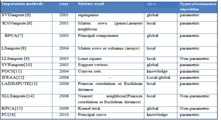
IV. EXISTING MISSING VALUE ESTIMATION METHODS
Several methods have been suggested to deal with the missing value problem .We have discussed here the existing missing value imputation methods and their performances taking the datasets being used into consideration.
One simple solution to the missing data problem is to repeat the experiment. This strategy can be expensive, but has been used in validation of microarray analysis algorithms. The other solution is to remove genes (rows) or experiments (columns) until no missing values exist. That means for a gene that has only a small number of missing values, we have to discard all the values in the corresponding row. This comes at a high price: we lose many observed values. Therefore, it’s desirable to estimate the missing values in order to analyse the available data.
Some of the generally applicable principles for estimating missing data are as follows:
A Mean Imputation
It is a simple procedure, in which the missing entries of the data matrix are estimated using the average of the non-missing values of the particular case or variable (row average or column average, respectively);
B. Hot Deck Imputation
It involves predicting missing values using similar non-missing cases, where the neighbourhood can be defined using a distance function or metric (the so-called nearest-neighbours hot deck);
C. Model Based Imputation It employs a statistical model. D. Multiple Imputation
This methods estimate more than one value for each missing entry.
E. Cold Deck Imputation
It uses an external source of information, such as data from other similar studies, to estimate the missing values
in the present study. Composite methods’ can also be defined that combine ideas from different approaches[5]. Different imputation algorithms have been classified into local approach, global approach, hybrid approach or knowledge assisted approaches based on the type of information used in the algorithm.
More advanced techniques, such as K-nearest neighbour method (KNNimpute) or the singular value decomposition method (SVDimpute), LS, LLS, IFRRA, has been developed. Now most recent methods are also present like projection onto convex set, kernelPCA, principal curves etc.
A. KNNimputation and SVDimputation
First we have discussed here the earliest methods such as KNNimpute and Singular Value Decomposition (SVD) imputation methods. For these method the data sets used by their characteristics: time series, noisy time series, and non-time series. Each data set is pre-processed for the evaluation by removing rows and columns containing missing expression values, yielding ‘complete’ matrices. The data are deleted at random to create test data sets. The estimation accuracy is based on Normalized Root Mean Squared (NRMS), difference between imputed matrix and the original matrix, divided by the average data value in the complete data set. This normalization allows for comparison of estimation accuracy between different data sets.
KNN-based method use nearest neighbor as parameter. Estimation method use is weighted average with Euclidean distance as metric. Euclidean distance measure is often sensitive to outliers, which could be present in microarray data. It has been found that log-transforming the data seems to sufficiently reduce the effect of outliers on gene similarity determination.
of missing values is used. Both the method does not utilize the correlation structure in the data.
B. Bayesian Principal Component Analysis
The estimation ability of KNN and SVDimpute methods depends on important model parameters, such as the k-value in KNNimpute and the number of eigenvectors in SVDimpute. There is no theoretical way, however, to determine these parameters appropriately. This is a global method consisting of three components. First, principal component regression, which is basically a low rank approximation of the data set, is performed. Second, Bayesian estimation, which assumes that the residual error and the projection of each gene on principal components behave as normal independent random variables with unknown parameters, is carried out. Third, Bayesian estimation follows by iterations based on the expectation-maximization (EM) of the unknown Bayesian parameters.The cDNA microarray data set relevant to the yeast cell-cycle as a complement has been used. This data set consists of three parts, which are relevant to alpha factor (A-part), elutriation (E-part), cdc15, and cdc28 (C-part) [7].
C. LSimpute
The second method utilizing the least squares principle to estimate missing values using correlations between genes and between array known as LSimpute.There are two basic LSimpute methods, one estimation method utilizing correlations between genes (LSimpute_gene) and the other using correlations between arrays as a basis for the estimation (LSimpute_array). Two variants of estimate combination that uses a bootstrapping approach for parameter (weight) estimation. The first, LSimpute_combined uses a fixed global weighting of the estimates from the basic LSimpute methods, while the second, LSimpute_adaptive, uses an adaptive weighting scheme taking the data correlation structure into consideration. Linear regression model for y given x as y = a + bx + e, where e is the error term for which the variance is minimized when estimating the model (parameters a and b) with least squares. The single regression model has two parameters to be estimated, while the multiple regression model has l (k + 1) parameters.
Here three data sets have been choosen from two cancer studies and one time series study. One data set comes from the NCI60 study. The second data set comes from a lymphoma study. The third data set is from an infection time series study. The LSimpute and has been compared with KNNimpute. While KNNimpute finds positively correlated genes by Euclidean distance, the LSimpute methods are able to include negative correlation between genes in the estimation model. LSimpute_combined and LSimpute_adaptive on data sets with 10% missing values reveals a root mean squared deviation(RMSD) between missing value estimates and the real values that is 15±20% smaller than that obtained using KNNimpute. LSimpute_gene gives a 4.4±9.7% smaller RMSD than
KNNimpute and LSimpute_array gives a 6.8±19.8% smaller RMSD with 5% missing values [8].
D. Local least squares imputation (LLSimpute)
In this method a target gene that has missing values is represented as a linear combination of similar genes. Rather than using all available genes in the data, only the gene with high similarity with the target gene has been used. LLSimpute takes advantage of the local similarity structures as well as the optimization process by the least squares, which is one of the most important advances of LLSimpute.
The data set being used was from a study of response to environmental changes in yeast. It contains 6361 genes and 156 experiments that have time-series of specific treatments.LLSimpute has been designed by estimating an optimal value i.e. the number of similar genes (k) used is 200. The NRMSE value for KNNimpute has been found to be 0.6 where as for LLSimpute it is reduced to 0.55[9]. One disadvantage of LLSimpute, however, is that the optimal number of neighbors is determined by a “heuristic” search which increases the computational cost of the algorithm.
E. Support vector regression (SVR)
Two kinds of Support Vector Machines are frequently used in practice: Support Vector machine for classification (SVC) and Support Vector machine for regression (SVR). Three kinds of kernel functions are often used in SVM, namely polynomial kernel function, radial basis kernel function and sigmoid kernel function, K (xi, x).The regression function of SVR is determined by the support vectors, the number of which is usually small when compared to the total number of the samples. Three different parameters is tuned for this kernel function.It is known that proper selection of parameter is very important for SVM, so the grid search strategy has been performed to find the best combination of parameters. The data sets used in this paper, one from Spellman’s work that focuses on identification of cell-cycle regulated genes in yeast Saccharomyces cerevisiae, an elutriation dataset as data E(time series data).Second one is from Gash’s experiment. Data G is a non-time-series data set when the percentage of entries missing is 20%, NRMSE of SVR impute reached 0.5611, while those of the other three methods KNNimpute, BPCAimpute and LLSimpute are 0.7762, 0.6615 and 0.7109, respectively for data E. When the percentage of entries missing is 10%, with NRMSE as low as 0.3135, while the NRMSE of the other methods in this condition are 0.5471, 0.3735 and 0.4045, respectively [10].
F. Projection onto convex sets (POCS)
the missing values into the estimation process to obtain an optimal result. The POCS algorithm conveniently combined both global and local information of both KNNimpute and SVDimpute to obtain a better solution. Two convex sets that are applicable to all microarray dataset have been introduced. They were constructed based on singular value decomposition. In addition, for the two most powerful missing value estimation methods KNNimpute and SVDimpute, there was a trade-off for whether to use a specific group of genes or to use all genes for missing value estimation. This algorithm can provide a best combination of these two strategies. To get the smoothest initial value for the time series dataset, the spline interpolation is used; while for non-time series dataset, the average of the gene expression profile is used. Datasets use here expression profiles for 6178 genes under different experimental conditions, i.e., cdc15, and cdc28, alpha factor and elutriation experiments POCS concludes that the NRMSE results of three missing value estimation methods when 10% of the data is missing, the algorithm can achieve 16-20% less error than the KNNimpute and SVDimpute[12].
G.Improved fixed rank approximation algorithm (IFRAA)
IFRAA is the improved FRAA [11].The disadvantage of FRAA that it does not perform as well as BPCA, KNNimpute and LLS. IFRAA is a combination of FRAA and a good clustering algorithm (such as k-means). FRAA is a robust algorithm which performs good, but not as well as KNNimpute. The KNNimpute is superior because it reconstructs the missing values of each gene from similar genes. IFRAA overcomes this disadvantage. First FRAA has been used to find a completion G (gene expression matrix with missing data) followed by cluster algorithm, (K-means by repeating and refining the cluster size), to find a reasonable number of clusters of similar genes. For each cluster of genes FRAA has been applied separately to recover the missing entries in this cluster. This modification has given a very efficient algorithm i.e. IFRAA for reconstructing the missing values of the gene expression matrix.
Six different types of data sets are used, consisting of four microarray gene expression data and two randomly
generated synthetic data. The first gene expression data set is a complete matrix of 5986 genes and 14 experiments based on the Elutriation data set in. The second microarray data set is based on Cdc15 data set in, which contains 5611 genes and 24 experiments. Two other yeast data sets are obtained from ”http://sgdlite.princeton.edu”. Other two are Evolution data set and Calcineurin data set. It has been found that for NRMSE value of IFRAA for Cdc15 data set %0.81 missing is 0.0175 where as for LLS,BPCA,FRAA ,it is 0.0200, 0.0216, 0.0335 respectively[12].
H. Least absolute deviation imputation(LAD impute) The proposed method uses the least absolute deviation to estimate the missing values using similarity measures. There are two LAD impute methods based on Euclidean distance (LAD impute/L2) or Pearson correlation coefficients (LAD impute/PC) between genes as similarity metric. Each missing value is initially estimated by the row average. Taking the first row in the dataset that contains missing entry as the target entity gt, k genes
gsi(i = 1, · · · , k)has been selected which are most similar to the target gene gt based on Pearson correlation coefficient or Euclidean distance. Using correlation among genes missing value(s) in gt has been computed by regression and then taking weighted average missing values are estimated.The dataset used here are the cDNA microarray data relevant to breast cancer, dataset from Elutriation block release that is studied for the identification of cell-cycle regulated genes in yeast Saccharomyces cerevisiae (SP ELU) and from a study of response to environmental changes in yeast (GASCH) .LAD impute (LAD impute/L2 and LAD impute/PC) has shown excellent performance over KNN method and LLSimpute for 5% missing data in gash is 0.65 where in KNN impute and LLSimpute it is nearly about 0.8.LAD impute method also reduces execution time for imputation. The previously developed KNNimpute method need to calculate nearest neighbours for each missing entry, while LAD impute imputes all missing values in a row simultaneously with given nearest neighbours[13].
I. Sequential local least squares imputation
The SLLSimpute method uses similar genes to estimate the missing values of the target gene and optimizes the estimation process with the least squares principle. In order to make the best use of the information available, the imputation is executed sequentially from the gene which has the least missing rate, and these sequentially imputed genes are used for the later imputation of the other genes. However, only genes with missing rate below a certain threshold are reused since genes with many imputed missing values are less reliable. SLLSimpute has been shown to exhibit better performance than LLSimpute due to the reuse of genes with missing values.
Four microarray data sets (SP.Alpha, YO.Calcineurin/Crzlp, RO.Cell-line and CU.Growth-regulator has been taken. The SLLSimpute has outperformed KNN-based imputation methods by incorporating the least squares principle, achieved an improvement over LLSimpute by introducing the sequential imputation procedure, and surpassed BPCAimpute by making good use of local similar structure existing in gene expression data. As the missing rate increases, utilization of the sequentially imputed data has not propagate errors as in the conventional LLSimpute method, thus SLLSimpute method has shown great improvement on both accuracy and stability compared with LLSimpute method[14].
J. Kernel PCA (KPCA)
Kernel principal component analysis (kernel PCA) is a generalization of standard PCA. It effectively exploits the “kernel trick” to find the features of observation data In kernel PCA regression, the regressors are not the observation data in the input space, but a nonlinear mapping of the observation data into the feature space. The regressors are thus called the features of the observation Data. To avoid non- linear mapping, a kernel function has been defined in the input space. A kernel matrix can be generated, of which each element is defined by the kernel function. The standard PCA has been performed on the kernel matrix such that the principal components of the features are first determined. They can be used as the regressors.
The first dataset (Dataset A) has been provided along with BPCA software with the size of 758 genes and 50 samples. The second dataset (Dataset B) was a breast cancer microarray from Stanford Microarray Database (SMD). Gaussian KPCAimpute performs best for Dataset A (when missing percent was 8%), comparing to the other two kernel PCA imputations. KPCAimpute algorithms outperform the BPCA and are similar to the LLSimpute (when 2% data was missing) for dataset B [15].
K.Principal curve(PC)
Principal curve is proposed by Hastie in 1984, which is an extension of principal component. Principal curve tries to find a smooth curve passing through the ’middle’ of all the data points. A curve can preserve more information about the structure of data distribution, and generally give better approximation than a line. Hastie defined the principal curves based on the conception of self-consistency. Self-consistency means that each point of the curve is the average of all points that project there. Thus a principal curve can provide a good one-dimensional nonlinear summary of the data .Principal curve algorithm has 2 steps- a projection step and an expectation step. The projection step computes projection indices of the data to the curve, and the expectation step constructs a new curve close to the ’middle’ of the data distribution.
The data sets used here are time series data such as α -factor, elutriation and arrest of a cdc15 temperature- sensitive mutant. This method has NRMSE error which is quite less than KNNimpute and LLSimpute with the missing percentage under 10%, and only a little less than BPCA for all the datasets[16].
V. DISCUSSION AND FUTURE DIRECTION There are many factors that can affect the performance of an imputation algorithm and there is probably no algorithm that performs the best in all data sets. Filling missing values with zeros or with average values over the cases are far from optimal solutions as they do not take into consideration the correlation structure in the data. The earliest imputation methods such as KNNimputation, LSimputation, and BPCAimputation etc are straightforward applications of the standard statistical imputation approaches to microarray data. Recently more application-specific modifications have been introduced such as POCS,KPCA,principal curve that take advantage of the particular properties of the data.In all of the discussed methods,they are compared at different percentages of missing data in terms of the similarity between the original and imputed data. The imputation accuracy is assessed using the root mean squared error (RMSE).The basic principle behind all the imputation method is by randomly removing certain percentage of data from the microarray dataset. First, a ’complete’ data set has been constructed by filtering the missing values.Then the imputation method has been run to estimate those missing value. The performance of the missing value estimation is evaluated by normalized root mean error (NRMSE). More accurate estimation brings smaller values of NRMSE.
LLSimputeare are determined in an ad hoc way without any theoretical foundation. BPCA is based on a strong statistical assumption and the numbers of principal axes are determined empirically. BPCA assumes only a global covariance structure; the estimation with BPCA may not be accurate if genes have dominant local similarity structures.LLSimpute takes advantage of the local similarity structures as well as the optimization process by the least squares, which is one of the most important advances of LLSimpute. LLSimpute has been shown to be highly competitive compared to KNNimpute and the much more complex BPCA.There have been some extensions to the basic LLSimpute algorithm like sequential LLSimpute (SLLSimpute) and iterated LLSimpute (ILLSimpute) .SVR mapping the samples into a much higher space which ensures the good performance of this method. POCS method is combined the merit of both KNN and SVDimputation.The two methods manifest an apparent trade-off between local and global information and their combination becomes an attractive alternative. In these developed methods the performance has deteriorated sharply as the number of missing values in the data set increases; some methods provide very different results when using different parameter values but there is no theoretical result for determining these parameters optimally. Parameter k in SLLSimpute method can be determined by a parameter selection algorithm automatically, it can be regarded as a non-parametric missing value estimation method. In order to distinguish from SLLSimpute with k-value uncertain, this non-parametric imputation method of SLLSimpute is referred to as SLLSkimpute.
LAD estimate is based on the assumption that the model has laplacian distributed errors. The previously developed KNNimpute method ,nearest neighbors for each missing entry is need to be calculated, while LADimpute imputes all missing values in a row simultaneously with given nearest neighbours. LAD estimate is not necessarily the best, since it does not require a tuning mechanism like most of the other robust regression procedures.The latter developed method, advantage of the KPCAimpute is that it has explored the features of the observed data and has used them as regressors in estimating missing values. Kernel PCA has been recently used in DNA microarray analysis, for example, in applications of gene expression data classification and clustering problems The Gaussian kernel has shown effective performance in the KPCAimpute.Next is the principal curve, by constructing principal curves, all the correlation information between different genes(samples) are integrated together also it has taken dynamic information along temporal axes into account via the computation of coordinate functions for principal curves. The combination of these two sources of information results in the performance improvement for this method.
In all the methods the case of missing at random has been considered. A real microarray data set usually has
non-random distribution of missing data. Missing not at random (MNAR), which is a more complex missing data mechanism, can be included in future research.Many missing value imputation methods have been developed for microarray data, but only a few studies have investigated the relationship between missing value imputation method and classification accuracy. We can investigate further how different properties of a dataset influence imputation and classification, and how imputation affects classification performance
VI. CONCLUSION
Missing values in microarray data can significantly affect subsequent analysis, thus it is important to estimate these missing values accurately . Existing microarray data analysis including data dimension reduction techniques, class prediction techniques, and clustering methods, however, often have difficulty in dealing with missing values. Many available algorithms for the statistical analysis of microarray data require a full data set without missing values, missing value imputation is an important pre-processing step in microarray data analysis. We have discussed some of the important imputation methods and their performance with respect to specific datasets, their strengths and also limitations. It is hoped that this comprehensive review would give the readers a better understanding of the current development in this field and inspire them to come up with the next generation of imputation algorithms.
REFERENCE
[1 ] Adi L. Tarca, Roberto Romero, and Sorin Draghici, “Analysis of microarray experiments of gene expression profiling “,American Journal of Obstetrics and Gynaecology (2006) 195, 373–88. [2] AlanWee-Chung Liew, Ngai-Fong Law and Hong Yan ” Missing
value imputation for gene expression data: computational techniques to recover missing data from available information “, Briefin in Bioinformatics,December,2010.
[3] Bhekisipho Twala, Motee Phorah, “Predicting incomplete gene microarray data with the use of supervised learning algorithms”, Pattern Recognition Letters, vol. 31,pp. 2061-2069,2010. [4] Anil K. Jain, Robert P.W. Duin, and Jianchang Mao, “Statistical
Pattern Recognition: A Review”,IEEE Trans. on Pattern Analysis and Machine Intelligence, vol. 22, no. 1,pp.4-36 January 2000. [5] Tero Aittokallio “Dealing with missing values in large-scale
studies: microarray data imputation and beyond”, Briefing in Bioinformatics,vol. 11, No 2,pp. 253-264,December.2009. [6] Troyanskaya O, Cantor M, Sherlock G, et al. Missing value
estimation methods for DNA microarrays,Bioinformatics, vol. 17(6),pp.520–525,2001.
[7] Oba S, Sato MA, Takemasa I,” A Bayesian missing value estimation method for gene expression profile data”, Bioinformatics ,vol.19,pp. 2088–2096,2003
[8] Trond Hellem Bù1, Bjarte Dysvik and Inge Jonassen “ LSimpute: accurate estimation of missing values in microarray data with least squares methods”, Nucleic Acids Research, vol. 32, No. 3 e34,pp. 1-8,2004.
[9] Kim H, Golub GH,and Park H. Missing value estimation for DNA microarray gene expression data: local least squares imputation” , IEEE Computational Systems Bioinformatics Conference (CSB 2004).
Medicine and Biology, 27th Annual Conference Shanghai, China, 2005,p. 6072.
[11] Xiangchao Gan, Alan Wee-Chung Liew and Hong Yan,” Missing Microarray Data Estimation Based on Projection onto Convex Sets Method”,in IEEE 17th International Conference on Pattern Recognition (ICPR’04) ,2004.
[12] Shmuel Friedland, Amir Niknejad, Mostafa Kaveh, and Hossein Zare,” An Algorithm for missing value estimation for DNA microarray data”, in ICASSP, 2006,vol. II,p. 1092.
[13] Yi Cao,and Kim Leng Poh,”An accurate and robust missing value estimation for Microarray data: least absolute deviation imputation”,in 5th International Conference on Machine Learning and Applications (ICMLA'06),2006.
[14] Zhang X, Song X, and Wang H, et al, “ Sequential local least squares imputation estimating missing value of microarray data”, Computers in Biology and Medicine, 2008,vol. 38,pp.1112–1120. [15] Ying Shan and Guang Deng ”Kernel PCA Regression for Missing Data Estimation in DNA Microarray Analysis”, IEEE Trans,pp. 1477-1480,2009.
[16] Jinlong Shi,and Zhigang Luo, “Missing value estimation for DNA microarray gene expression data with principal curves “,in International Conference on Bioinformatics and Biomedical Technology,pp. 262-265,2010.
[17] Tobias K. Karakach,Robert M. Flight ,Susan E. Douglas ,and Peter D. Wentzell, “An introduction to DNA microarrays for gene expression analysis” , Chemometrics and Intelligent Laboratory
Systems,2010