An Ensemble Method with Sentiment Features and Clustering Support
Nguyen Huy Tien
Japan Advanced Institute of Science and Technology (JAIST)
Nguyen Minh Le
Japan Advanced Institute of Science and Technology (JAIST)
Abstract
Deep learning models have recently been applied successfully in natural language processing, especially sentiment analysis. Each deep learning model has a particu-lar advantage, but it is difficult to com-bine these advantages into one model, es-pecially in the area of sentiment analy-sis. In our approach, Convolutional Neu-ral Network (CNN) and Long Short Term Memory (LSTM) were utilized to learn sentiment-specific features in a freezing scheme. This scenario provides a novel and efficient way for integrating advan-tages of deep learning models. In addi-tion, we also grouped documents into clus-ters by their similarity and applied the pre-diction score of Naive Bayes SVM (NB-SVM) method to boost the classification accuracy of each group. The experiments show that our method achieves the state-of-the-art performance on two well-known datasets: IMDB large movie reviews for document level and Pang & Lee movie re-views for sentence level.
1 Introduction
The emergence of web 2.0, which allows users to generate content, is causing the rapid increase in the amount of data. This platform, which enables millions of users to share information and com-ments, has a high demand for extracting knowl-edge from user-generated content. An important information to be analyzed from those comments is opinions/sentiments, which express subjective opinions of particular users. Sentiment analysis is a fundamental task and has attracted a huge amount of research in recent years (Pang and Lee, 2008;Liu,2012). The task calls for identifying the
sentiment polarity (positive, negative) of a com-ment or review.
Wang (2012) used a Support Vector Machine variant with Naive Bayes feature (NBSVM). Pre-senting a document or a sentence with Bag of bi-gram features, NBSVM consistently performs well across datasets of long and short reviews. Recently, the success of deep learning in natu-ral language processing has led to many efficient methods for sentiment analysis such as Paragraph Vector (Le and Mikolov, 2014), CNN (Kalch-brenner et al.,2014;Kim,2014;Zhang and Wal-lace,2015), LSTM (Wang et al.,2015;Liu et al., 2015). In Paragraph Vector, Le and Mikolov em-ployed the technique of Word embedding repre-sentation using neural networks (Bengio et al., 2003;Collobert and Weston,2008;Mnih and Hin-ton, 2009; Turian et al., 2010; Mikolov et al., 2013) to represent a document or paragraph as a vector. This document modeling outperformed the Bag of Words model in sentiment analysis and in-formation retrieval. Li (2015) has enhanced the architecture of Paragraph Vector by allowing the model to predict not only words but also n-gram features (DVngram). CNN is capable of capturing local relationships between neighbor words in a sentence but fails for long-distance dependencies. LSTM can handle CNN’s limitation because it is able to memorize information for a long period of time. Our motivation is to build a combination ap-proach taking the advantages of these methods.
In this paper, we separately designed CNN and LSTM models to encode sentiment informa-tion into feature vectors. To apply for senti-ment classification, these sentisenti-ment-specific vec-tors and the semantic-specific DVngram vector were passed into the 3-layer neural network. In sentiment analysis, two sentences with a slight dif-ference could provide opposite sentiments. Gener-ative models, however, have a tendency to encode
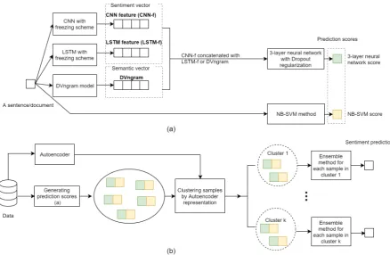
Figure 1: The proposed framework for sentiment analysis
similar sentences/documents into similar vectors. For that reason, we designed an autoencoder model to learn representation vectors for sen-tences/documents and used these vectors for clus-tering. The prediction score of NBSVM method is provided to enhance the sentiment prediction of each cluster. Figure 1 shows the architecture of our framework.
We compared our method with NBSVM, CNN, LSTM, Paragraph Vector, LinearEnsemble (Mes-nil et al., 2014), DSCNN (Zhang et al., 2016) on three well-known datasets: IMDB large movie reviews (Maas et al., 2011) for document level, Pang & Lee (2005) movie reviews and Stanford Sentiment Treebank (Socher et al.,2013) for sen-tence level. The experimental results show that our method consistently performs well on both docu-ment and sentence level data. The main contribu-tions of this work are as follows:
• We applied a freezing scheme to CNN and LSTM models for encoding sentiment infor-mation into vectors. These vectors provide a simple and efficient way to integrate the strong abilities of deep learning models.
• We proposed a scenario to divide data into groups of similar sentences/documents.
Then, each sentence/document in each group is represented by the prediction score of NB-SVM method and the prediction score of the proposed 3-layer neural network. We pro-posed an ensemble method to employ these scores.
2 Sentiment representation learning In this section, we describe the freezing scheme to generate sentiment vectors from two models: (i) CNN, (ii) LSTM; and a method to employ these vectors. To feed into LSTM/CNN model, each word of a sentence/document is transformed into a word embedding vector usingWord2Vec1.
Le and Mikolov(2014) extended the word em-bedding learning model by incorporating para-graph information. Given a paragraph, Le’s method captures and encodes semantics into a rep-resentation vector or a semantic feature.
This work inspired us to develop a document representation learning model to capture senti-ment information. In our work, we proposed an approach to generating sentiment representation from CNN and LSTM models. Our idea is to train CNN and LSTM models under the sentiment clas-sification task. In a deep learning network, we
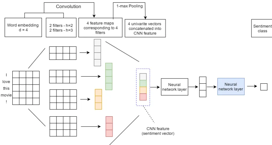
Figure 2: Illustration of our CNN framework to generate sentiment features. Given a sequence ofd -dimension word embeddings (d= 4), the model applies 4 filters: 2 filters for region sizeh = 2and 2 filters for region sizeh = 3to generate 4 feature maps. During the training process, the parameters of the last neural network layer (blue one) are frozen (untrained)
could separate the model into two parts: (i) Build-ing target feature- from input samples, the first part encodes target information into vectors, (ii) Classifying layer - the second part tries to learn a layer (or a boundary) for classifying these vec-tors into target labels. Sentiment vecvec-tors gener-ated by a model, however, are much fitting to the classifying layer of this model. It is not efficient to combine two sentiment vectors generated from two models because each sentiment vector is fit-ting to its particular classifying layer. To address this problem, we proposed a freezing scheme. Ac-cording to this scheme, the parameters of the clas-sifying layer are initialized from the uniform dis-tribution and in the training phase, these param-eters are kept unchanged. This technique makes sentiment vectors not too fit to a particular classi-fying layer.
2.1 LSTM for sentiment feature engineering - LSTM feature
The LSTM architecture was introduced by Hochreiter (1997). By designing a memory cell preserving its state over a long period of time and non-linear gating units regulating information flow into and out of the cell, Hochreiter made LSTM able to capture efficiently long distance
de-Figure 3: Illustration of our LSTM model to gen-erate sentiment vectors. During the training pro-cess, the parameters of the neural network layer (blue one) are frozen (untrained)
pendencies of sequential data without suffering the exploding or vanishing gradient problem of Recur-rent neural network (Goller and Kuchler,1996).
over sequential data. The model contains two parts: (i)Building sentiment feature- the LSTM layer encodes sentiment information of input into a fixed-length vector; (ii)Classifying layer- this sentiment-specific representation vector will be classified by the last neural network (NN) layer (the blue layer in Figure3). As applying the freez-ing scheme, this NN layer’s parameters are un-changed during the training process.
2.2 CNN for sentiment feature engineering -CNN feature
We present a sentence of lengthsas a matrixd×s, where each row is ad-dimension word embedding vector of each word. Given a sentence matrixS, CNN performs convolution on this input via lin-ear filters. A filter is denoted as a weight ma-trix W of length d and region size h. W will have d×h parameters to be estimated. For an input matrix S ∈ Rd×s, a feature map vector
O = [oo, o1, ..., os−h] ∈ Rs−h+1 of the convo-lution operator with a filterW is obtained by ap-plying repeatedlyW to sub-matrices ofS:
oi =W ·Si:i+h−1 (1)
wherei= 0,1,2, ..., s−h, (·) is dot product and
Si:j is the sub-matrix of S from rowitoj. Each feature mapOis fed to a pooling layer to generate potential features. The common strategy is 1-max pooling (Boureau et al.,2010). The idea of 1-max pooling is to capture the most important feature v corresponding to the particular feature map by selecting the highest value of that feature map:
v= max
0≤i≤s−h{oi} (2) We have described in detail the process of one filter. Figure 2 shows an illustration of apply-ing multiple filters with variant region sizes to ob-tain multiple 1-max pooling values. After pooling, these 1-max pooling values from feature maps are concatenated into a CNN feature carrying senti-ment information. Intuitively, the CNN feature is a collection of maximum values from the feature maps. To make a connection to these values, we provide an NN layer to synthesize a high-level fea-ture from the CNN feafea-ture. Finally, this high-level feature is passed to an NN layer with sigmoid acti-vation to generate the probability distribution over sentiment labels.
In the training phase, similar to the strategy in our LSTM model, the last NN layer’s parameters
are kept untrained to make the sentiment vectors not too fit to a particular classifying layer.
2.3 Classifying with sentiment vectors
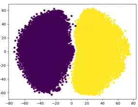
Figure4 visualizes the results of encoding senti-ments into vectors using our CNN model. As we can see in the development set, there are some un-ambiguous cases. Therefore, we add more infor-mation to CNN sentiment vectors by concatenat-ing them with LSTM sentiment vectors or DVn-gram semantic vectors.
As CNN and LSTM sentiment vectors are, how-ever, generated from models of sentiment clas-sification, these vectors are easily separated in terms of sentimental categories by machine learn-ing methods. In other words, a multi-layer NN sentiment classifier using both of these vectors as input reaches the state of perfect classification on the training set after a few epochs. In this case, the classifier’s parameters are not efficiently opti-mized and the classifier’s performance has no im-provement on the testing set, compared with using LSTM or CNN for classification (or we call the model overfitting).
To address this problem, we employ a3-layer NN with Dropout regularization (Hinton et al., 2012) on the first and second layers. By randomly dropping out each hidden unit with a probabil-ity p on each presentation of each training case, Dropout prevents overfitting and provides a way to combine many variant NN architectures effi-ciently. By applying Dropout, our model has an ability to examine efficiently variant combination ways from feature vectors.
(a) Sentiment vectors in the train set
(b) Sentiment vectors in the development set Figure 4: The t-SNE projection for IMDB dataset’s sentiment vectors (positive and negative) generated from our CNN model.
each cluster, the prediction score of the method in section 2 are combined with the prediction score of NBSVM. The reason for choosing NBSVM is that NBSVM is an efficient method not based on neutral network architectures, and using Bag of Word model to represent sentences/documents, which is different from the word embedding repre-sentation. We consider NBSVM’s score as an ad-ditional channel and expect it to support well for each group of similarity sentences/documents in terms of word embedding representation.
Given a sentence/document, we will have two prediction scores: one from the proposed method in section 2 and one from NBSVM. To employ these scores, we used a voting method. This scheme allows each classifierfito give a vote with a confident ratio ri to the final probability score over classes distribution as follows:
p(ci|x) = N1 N
X
k=1
pk(ci|x)rk (3)
whereci is theith sentiment class, N is the num-ber of classifiers, pk(ci|x) is the prediction score of the classifier k on the ith class for a sen-tence/documentx.
(a) BiLSTM model
(b) CNN model. In MR-L dataset, each region size has 300 filters. In MR-S and SST dataset, each region size has 100 filters
Figure 5: Autoencoder models
The objective of this ensemble method is to se-lect a suitable confident ratio for each classifier to optimize the performance of classification. In our approach, a 2-layer NN is employed to define a voting architecture. We consider a feedforward process in NN as a scheme of voting and the NN’s weights as confident ratios. Adamax algorithm (Kingma and Ba,2014) is applied to optimize the weights of the model.
Dataset l train test |V| MR-L 300 25000 25000 169940
MR-S 20 10662 cv 18765
SST 19 9613 1821 16185
Table 1: Summary statistic of datasets. ldenotes the average length of reviews,trainandtestare sizes of the training set and the test set respec-tively, cv is 10-fold cross validation, and |V| is vocabulary size.
4 Dataset and Experiment setup 4.1 Dataset
We evaluated our models on three well-known datasets. Table 1shows the statistic summary of datasets.
• For document level, IMDB large movie re-view datasetMR-Lis used. Each review con-tains numerous sentences (Maas et al.,2011).
movie review. In addition, we also did exper-iment on Stanford Sentexper-iment TreebankSST (Socher et al., 2013) - an extension of MR-S with two labels (positive and negative). In SST, all sentences and phrases of the training set are used for training.
4.2 Experimental setup
To tune hyper-parameters of our models, we do a grid search on 30% of each dataset.
• For MR-L:
– LSTM model has dimensiond= 32. – CNN model: using 3 region sizes of
3,4,5; the number of each region size is300and the dimension of penultimate NN layer is 100.
– 3-layer NN model for classification with sentiment vectors: the first NN layer has the same dimension as the input feature, and the dropout ratio p = 0.9; the sec-ond NN layer has the dimension of 64 and the dropout ratiop= 0.5.
– Autoencoder models: we examined two autoencoder models - CNN and BiL-STM. The details are in Figure5. – Clustering: k-mean is applied. The
number of clusters isk= 2.
– Ensemble model: the first NN layer has the dimension of 3×the input’s dimen-sion or the number of classifiers.
• For MR-S and SST: the same configuration as MR-L, except the number of each region size is100.
For word vectors, we obtained pre-trained word vectorsWord2Vec. Its vectors have the dimension of 300. In our LSTM and CNN models, these pre-trained word vectors are optimized during the training process.
5 Results and Discussion
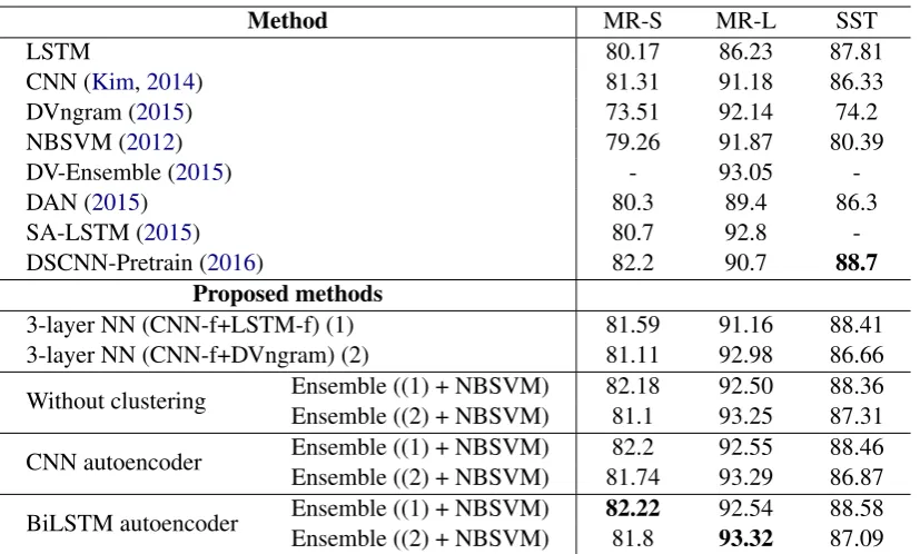
We compared our models against the other meth-ods showed in table2on the binary sentiment clas-sification task. In SST dataset, we could not re-produce the result 88.1% of CNN (Kim, 2014). According to the empirical results, our method of combining feature vectors 3-layer NN outper-forms the individual methods: LSTM, CNN, and
DVngram. That proves the efficiency of the fea-ture combination strategy. In addition, our en-semble method with clustering support outper-forms the current state of the art method on MR-L and MR-S datasets. As we mentioned in Sec-tion 3, NBSVM uses a different way to present sentences/documents and a different approach to learning (a discriminative model), so it gives a significant support in our ensemble method. On document level, LSTM method produced a much lower performance than DVngram method. As a result, the feature vectors generated from LSTM model does not support as well as DVngram’s vec-tors when combining with CNN feature vecvec-tors. 5.1 Freezing vs Unfreezing in the last NN
layer of feature engineering phase
In the engineering phase, we freeze (untrain) the last NN layer’s parameters to create efficient sen-timent vectors. To evaluate the efficiency of this technique, we compared our vector’s perfor-mance against the sentiment-specific vector from the unfreezing scheme. We passed these vec-tors to our 3-layer NN model to achieve the re-sults (details in table 3). One interesting obser-vation is that the performance of a feature vec-tor in freezing mode is better than one in un-freezing mode for most of the cases. In addition, we combined a sentiment-specific vector with the semantic-specific vector - DVngram for evaluating the performance. In general, our freezing scheme provided a higher performance than the unfreez-ing scheme. The experimental results show that our freezing scheme works more efficiently on CNN model than LSTM model, especially in a case of combining a sentiment-specific vector and a semantic-specific vector.
5.2 Evaluation on combining features
In this section, we compared in performance our approach to combining features from variant mod-els against Merging scheme which horizontally merges variant models (details in figure6).
Merg-Method MR-S MR-L SST
LSTM 80.17 86.23 87.81
CNN (Kim,2014) 81.31 91.18 86.33
DVngram (2015) 73.51 92.14 74.2
NBSVM (2012) 79.26 91.87 80.39
DV-Ensemble (2015) - 93.05
-DAN (2015) 80.3 89.4 86.3
SA-LSTM (2015) 80.7 92.8
-DSCNN-Pretrain (2016) 82.2 90.7 88.7
Proposed methods
3-layer NN (CNN-f+LSTM-f) (1) 81.59 91.16 88.41
3-layer NN (CNN-f+DVngram) (2) 81.11 92.98 86.66
Without clustering Ensemble ((1) + NBSVM)Ensemble ((2) + NBSVM) 82.1881.1 92.5093.25 88.3687.31
CNN autoencoder Ensemble ((1) + NBSVM)Ensemble ((2) + NBSVM) 81.7482.2 92.5593.29 88.4686.87
BiLSTM autoencoder Ensemble ((1) + NBSVM)Ensemble ((2) + NBSVM) 82.2281.8 92.5493.32 88.5887.09
Table 2: Accuracy results on the binary sentiment classification task. 3-layer NN(F1 +F2) denotes using feature vectorF1andF2as input;CNN-f,LSTM-fdenote sentiment-specific feature vectors gen-erated from the proposed CNN, LSTM respectively;Ensemble(p1+p2)denotes applying the proposed Ensemble for the prediction scores ofp1andp2.
Feature MR-S MR-L SST
CNNorg 80.61 91.22 86.05
CNN-f 80.89 91.38 86.27
LSTMorg 78.97 85.5 86.99
LSTM-f 79.11 85.14 87.64
CNNorg + LSTMorg 80.95 90.34 87.31 CNN-f + LSTM-f 81.59 91.16 88.41 CNNorg + DVngram 80.6 92.66 85.34 CNN-f + DVngram 81.11 92.98 86.66 LSTMorg + DVngram 79.38 90.41 87.2 LSTM-f + DVngram 79.59 88.04 88.14
Table 3: Accuracy results of 3-layer NN method on different features.CNNorg,LSTMorgdenote sentiment-specific features engineering from the proposed CNN, LSTM without freezing the last NN layer respectively
Method MR-S MR-L SST
3-layer NN (CNN-f + LSTM-f) 81.59 91.16 88.41
CNN-LSTM 81.07 91.07 86.49
3-layer NN (CNN-f + DVngram) 81.11 92.98 86.66
CNN-DVngram 80.79 92.12 85.39
3-layer NN (LSTM-f + DVngram) 79.59 88.04 88.14
LSTM-DVngram 80.61 92.08 86.49
Table 4: Accuracy results of features combining scheme and Merging scheme.
ing scheme). In most of the cases in Merging scheme, a composition model (i.e. CNN-LSTM) try to reproduce the result of its child models (e.g. CNN, LSTM) and does not provide a significant improvement.
Figure 6: The architecture of merging models.
5.3 Error analysis
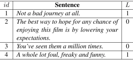
To get a better sense of the limitation of the pro-posed model, we manually inspect some cases of the wrong prediction, which are showed in table 5. These sentences are good examples of the pro-posed model’s weakness.
The second reason of the wrong prediction comes from missing context information. A word (i.g. foul, freaky) carries a positive or negative senti-ment depend on context or domains. We believe that the promising direction in future work will be to improve the model for capturing syntactic and context information.
id Sentence L
1 Not a bad journey at all. 1
2 The best way to hope for any chance of enjoying this film is by lowering your expectations.
0
3 You’ve seen them a million times. 0 4 A whole lot foul, freaky and funny. 1
Table 5: Examples of the wrong prediction.L de-notes the true label with 0,1 for negative, positive sentiment labels respectively)
6 Related work
Sentiment analysis is a study of determining people’s opinions, emotions toward to entities. Taboada (2011) assigned sentiment labels to text by extracting sentiment words. Liu (2012) formu-lated the sentiment analysis as a classification task and applied machine learning techniques for this problem. In this approach, dominant research con-centrated on designing effective features such as word ngram (Wang and Manning,2012), emoticon (Zhao et al.,2012), sentiment words (Kiritchenko et al., 2014). However, designing handcraft fea-tures requires an intensive effort.
Recently, the emergence of deep learning mod-els has provided an efficient way to learn contin-uous representation vectors for sentiment classi-fication. Bengio (2003) and Mikolov (2013) in-troduced learning techniques for semantic word representation. By using a neural network in the context of a word prediction task, the authors gen-erated word embedding vectors carrying seman-tic meanings. Embedding vectors of words which share similar meanings are close to each other. Se-mantic information maybe provides opposite opin-ions in different contexts. Therefore, some re-search (Socher et al., 2011; Tang et al., 2014) worked on learning sentiment-specific word rep-resentation by employing sentiment text. For sen-tence and document level, composition approach attracted many studies. Yessenalina and Cardie (2011) modeled each word as a matrix and used
iterated matrix multiplication to present a phrase. Deep recursive neural networks (DRNN) over tree structures were employed to learn sentence rep-resentation for sentiment classification such as DRNN with binary parse trees (Irsoy and Cardie, 2014), Recursive tensor neural network with sen-timent treebank (Socher et al.,2013). CNN has re-cently been applied efficiently for semantic com-position (Kim, 2014;Zhang and Wallace, 2015). This technique uses convolutional filters to capture local dependencies in term of context windows and applies a pooling layer to extract global fea-tures. Le and Mikolov (2014) applied paragraph information into the word embedding technique to learn semantic representation. Tang et al. (2015) used CNN or LSTM to learn sentence representa-tion and encoded these semantic vectors in docu-ment representation by Gated recurrent neural net-work. Zhang (2016) proposed Dependency Sen-sitive CNN to build hierarchically textual repre-sentations by processing pretrained word embed-dings. Wang (2016) used a regional CNN-LSTM to predict the valence arousal ratings of texts.
In our work, we designed a freezing approach for learning efficiently sentiment document rep-resentation from two variant deep-learning mod-els: CNN and LSTM. Afterward, these sentiment-specific vectors and the semantic DVngram vector were employed for sentiment classification. This strategy captures the advantages of variant models by using vectors, which each model generated. We also used NBSVM in clustering mode to boost the performance of classification.
7 Conclusion
References
Yoshua Bengio, R´ejean Ducharme, Pascal Vincent, and Christian Jauvin. 2003. A neural probabilistic lan-guage model. journal of machine learning research, 3(Feb):1137–1155.
Y-Lan Boureau, Jean Ponce, and Yann LeCun. 2010. A theoretical analysis of feature pooling in visual
recognition. In Proceedings of the 27th
interna-tional conference on machine learning (ICML-10), pages 111–118.
Ronan Collobert and Jason Weston. 2008. A unified architecture for natural language processing: Deep
neural networks with multitask learning. In
Pro-ceedings of the 25th international conference on Machine learning, pages 160–167. ACM.
Andrew M Dai and Quoc V Le. 2015. Semi-supervised
sequence learning. InAdvances in Neural
Informa-tion Processing Systems, pages 3079–3087.
Christoph Goller and Andreas Kuchler. 1996. Learning task-dependent distributed representations by
back-propagation through structure. InNeural Networks,
1996., IEEE International Conference on, volume 1, pages 347–352. IEEE.
Geoffrey E Hinton, Nitish Srivastava, Alex Krizhevsky, Ilya Sutskever, and Ruslan R Salakhutdinov. 2012. Improving neural networks by preventing
co-adaptation of feature detectors. arXiv preprint
arXiv:1207.0580.
Sepp Hochreiter and J¨urgen Schmidhuber. 1997.
Long short-term memory. Neural computation,
9(8):1735–1780.
Ozan Irsoy and Claire Cardie. 2014. Deep recursive neural networks for compositionality in language. InAdvances in Neural Information Processing
Sys-tems, pages 2096–2104.
Mohit Iyyer, Varun Manjunatha, Jordan L Boyd-Graber, and Hal Daum´e III. 2015. Deep unordered composition rivals syntactic methods for text classi-fication. InACL (1), pages 1681–1691.
Nal Kalchbrenner, Edward Grefenstette, and Phil
Blunsom. 2014. A convolutional neural
net-work for modelling sentences. arXiv preprint
arXiv:1404.2188.
Yoon Kim. 2014. Convolutional neural
net-works for sentence classification. arXiv preprint
arXiv:1408.5882.
Diederik Kingma and Jimmy Ba. 2014. Adam: A
method for stochastic optimization. arXiv preprint
arXiv:1412.6980.
Svetlana Kiritchenko, Xiaodan Zhu, and Saif M Mo-hammad. 2014. Sentiment analysis of short in-formal texts. Journal of Artificial Intelligence Re-search, 50:723–762.
Quoc V Le and Tomas Mikolov. 2014. Distributed
rep-resentations of sentences and documents. InICML,
volume 14, pages 1188–1196.
Bofang Li, Tao Liu, Xiaoyong Du, Deyuan Zhang, and Zhe Zhao. 2015. Learning document embed-dings by predicting n-grams for sentiment
classi-fication of long movie reviews. arXiv preprint
arXiv:1512.08183.
Bing Liu. 2012. Sentiment analysis and opinion min-ing. Synthesis lectures on human language tech-nologies, 5(1):1–167.
Pengfei Liu, Shafiq Joty, and Helen Meng. 2015. Fine-grained opinion mining with recurrent neural
net-works and word embeddings. In Conference on
Empirical Methods in Natural Language Processing (EMNLP 2015).
Andrew L. Maas, Raymond E. Daly, Peter T. Pham, Dan Huang, Andrew Y. Ng, and Christopher Potts.
2011. Learning word vectors for sentiment
analy-sis. InProceedings of the 49th Annual Meeting of the Association for Computational Linguistics: Hu-man Language Technologies, pages 142–150, Port-land, Oregon, USA. Association for Computational Linguistics.
Gr´egoire Mesnil, Tomas Mikolov, Marc’Aurelio
Ran-zato, and Yoshua Bengio. 2014. Ensemble of
generative and discriminative techniques for
senti-ment analysis of movie reviews. arXiv preprint
arXiv:1412.5335.
Tomas Mikolov, Kai Chen, Greg Corrado, and
Jef-frey Dean. 2013. Efficient estimation of word
representations in vector space. arXiv preprint
arXiv:1301.3781.
Andriy Mnih and Geoffrey E Hinton. 2009. A scal-able hierarchical distributed language model. In
Advances in neural information processing systems, pages 1081–1088.
Bo Pang and Lillian Lee. 2005. Seeing stars: Exploit-ing class relationships for sentiment categorization with respect to rating scales. InProceedings of the ACL.
Bo Pang and Lillian Lee. 2008. Opinion mining and sentiment analysis. Foundations and trends in infor-mation retrieval, 2(1-2):1–135.
Richard Socher, Jeffrey Pennington, Eric H Huang, Andrew Y Ng, and Christopher D Manning. 2011. Semi-supervised recursive autoencoders for
predict-ing sentiment distributions. In Proceedings of the
Conference on Empirical Methods in Natural Lan-guage Processing, pages 151–161. Association for Computational Linguistics.
for semantic compositionality over a sentiment tree-bank. InProceedings of the conference on empirical methods in natural language processing (EMNLP), volume 1631, page 1642. Citeseer.
Maite Taboada, Julian Brooke, Milan Tofiloski, Kim-berly Voll, and Manfred Stede. 2011. Lexicon-based
methods for sentiment analysis. Computational
lin-guistics, 37(2):267–307.
Duyu Tang, Bing Qin, and Ting Liu. 2015. Document modeling with gated recurrent neural network for sentiment classification. InProceedings of the 2015 Conference on Empirical Methods in Natural Lan-guage Processing, pages 1422–1432.
Duyu Tang, Furu Wei, Nan Yang, Ming Zhou, Ting Liu, and Bing Qin. 2014. Learning sentiment-specific word embedding for twitter sentiment clas-sification. InACL (1), pages 1555–1565.
Joseph Turian, Lev Ratinov, and Yoshua Bengio. 2010. Word representations: a simple and general method for semi-supervised learning. InProceedings of the 48th annual meeting of the association for compu-tational linguistics, pages 384–394. Association for Computational Linguistics.
Jin Wang, Liang-Chih Yu, K Robert Lai, and Xuejie Zhang. 2016. Dimensional sentiment analysis
us-ing a regional cnn-lstm model. InThe 54th Annual
Meeting of the Association for Computational Lin-guistics, volume 225.
Sida Wang and Christopher D Manning. 2012. Base-lines and bigrams: Simple, good sentiment and topic
classification. In Proceedings of the 50th Annual
Meeting of the Association for Computational Lin-guistics: Short Papers-Volume 2, pages 90–94. As-sociation for Computational Linguistics.
Xin Wang, Yuanchao Liu, Chengjie Sun, Baoxun Wang, and Xiaolong Wang. 2015. Predicting po-larities of tweets by composing word embeddings
with long short-term memory. InProceedings of the
53rd Annual Meeting of the Association for Compu-tational Linguistics and the 7th International Joint Conference on Natural Language Processing, vol-ume 1, pages 1343–1353.
Ainur Yessenalina and Claire Cardie. 2011. Compo-sitional matrix-space models for sentiment
analy-sis. In Proceedings of the Conference on
Empiri-cal Methods in Natural Language Processing, pages 172–182. Association for Computational Linguis-tics.
Rui Zhang, Honglak Lee, and Dragomir Radev. 2016. Dependency sensitive convolutional neural networks
for modeling sentences and documents. arXiv
preprint arXiv:1611.02361.
Ye Zhang and Byron Wallace. 2015. A sensitivity anal-ysis of (and practitioners’ guide to) convolutional
neural networks for sentence classification. arXiv
preprint arXiv:1510.03820.
Jichang Zhao, Li Dong, Junjie Wu, and Ke Xu. 2012. Moodlens: an emoticon-based sentiment analysis
system for chinese tweets. In Proceedings of the