Some New Solutions of Shallow Water Wave
Equation with Variable Coefficients By Generalized
(
G
′G
)
-Expansion Method
Lakhveer Kaur
11
Department of Mathematics, AIAS
Amity University, Noida (Uttar Pradesh), INDIA
Abstract
In this work, the generalized
(
G′ G
)
-expansion method is presented to seek some new exact solutions of Shallow Water wave equation with variable coefficients. As a result, more explicit traveling wave solutions involving arbitrary param-eters are found out, which are expressed in terms of hyperbolic functions, the trigonometric functions and rational functions. When the parameters are taken special values, different types of wave solutions can be obtained.
.
Keywords: Variable Coefficients Shallow Water Wave equation, Generalized
(G′
G
)
-Expansion method, Exact Solutions.
(2010) Mathematics Subject Classification:35Q99, 35C09, 35A25, 83C15.
1
Introduction
The nonlinear partial differential equations in mathematical physics have played a major role in a great variety of contexts, such as physics, biology, engineering, fluid flow, signal processing, system identification, control theory, finance, and fractional dynamics. Wide classes of analytical methods have been proposed for finding the exact solutions of these nonlinear partial differential equations. For integrable non-linear differential equations, the inverse scattering transform method [1], the Hirota method [2], the truncated Painlev´e expansion method [3], the B¨acklund transform method [4, 5] and the exp-function method [6, 7, 8] are used in looking for the exact solutions of nonlinear partial differential equations. Among non-integrable nonlinear differential equations, there is a wide class of the equations that referred to as the partially integrable, because these equations become integrable for some values of
1Corresponding author:
their parameters. There are many different methods to look for the exact solutions of these equations. The most famous algorithms are the Weierstrass elliptic function function method [9], the tanh- function method [10, 11]and the Jacobi elliptic func-tion expansion method [12, 13] and so on.
However to our knowledge, most of aforementioned methods are related to the con-stant coefficient models. But the physical situations in which nonlinear equations arise tend to be highly idealized because of assumption of constant coefficients. Be-cause of this, the study of nonlinear equations with variable coefficients has attracted much attention [14, 15, 16].
Among the other methods, a new method called Generalized(G′ G
)
- Expansion method [17, 18] has been proposed to seek exact solutions of nonlinear partial differential equations. Being concise and straightforward, this method can be applied to various nonlinear partial differential equations with variable coefficients. As a result, hyper-bolic function solutions, trigonometric function solutions and rational solutions with various parameters are obtained.
This method is based on the assumptions that the traveling wave solutions can be expressed by a polynomial in (GG′) where G = G(θ) satisfies the following second order linear ordinary differential equation
G′′(θ) +λG′(θ) +µG(θ) = 0, (1.1)
where θ=p(t)x+q(t), p(t) andq(t) are functions to be determined.
This paper is organized as follows: In section 2, we summarize the generalized (GG′) -expansion method. We apply the method to physically important nonlinear evolution equation, namely, shallow water wave equation with variable coefficients in section 3 and abundant exact solutions are obtained which included the hyperbolic func-tions, the trigonometric functions and rational functions. Finally, we record some concluding remarks in last section.
2
Description of The Generalized
(
G′G
)
-Expansion
Method [17]
Consider the nonlinear partial differential equation with independent variables X = (x, y, z, ..., t) and dependent variable u in the following form:
F(u, ut, ux, uy, uz, ...uxt, uyt, uzt, utt, ...) = 0, (2.1)
whereu=u(x, y, z, ...t) is an unknown function,F is a polynomial inu=u(x, y, z, ...t) and its various partial derivatives, in which the highest order derivatives and nonlin-ear terms are involved. In the following, we give the main steps of the generalized
(G′
G
)
-expansion method.
Step 1: We suppose that the solution of Eq. (2.1) can be expressed by a polynomial in(GG′) as follows:
u=α0(X) +
m
∑
i=1
αi(X)
(
G′ G
)i
, αm(X)̸= 0, (2.2)
0 i
determined later and G=G(θ) satisfies following equation
G′′(θ) +λG′(θ) +µG(θ) = 0, (2.3)
where θ=p(t)x+q(t), p(t) andq(t) are functions to be determined.
Step 2: In order to determine u explicitly, we firstly find the value of integer m by balancing the highest order nonlinear term(s) and the highest order partial derivative of u in Eq. (1.1).
Step 3: Substitute (2.2) along with Eq. (2.3) into Eq. (2.1) and collect all terms with the same order of(GG′)together, the left hand side of Eq. (2.1) is converted into a polynomial in(GG′). Then by setting each coefficient of this polynomial to zero, we derive a set of over-determined partial differential equations for α0(X), αi(X) and ζ.
Step 4: Solve the system of over-determined partial differential equations obtained in Step 3 for α0(X), αi(X) and ζ.
Step 5: Use the results obtained in above steps to derive the solutions of Eq. (2.1) depending on (G′
G
)
, since the solutions of Eq. (2.3) have been well known to us depending on the sign of the discriminant ∆ = λ2−4µ, then the exact solutions of
Eq. (2.1) are furnished.
3
Application of Generalized
(
G′G
)
-Expansion Method
to Shallow Water Wave Equation with Variable
Coefficients
In this section, we will use generalized (GG′)-expansion method to derive certain new solutions of shallow water wave equation with variable coefficients, which is very important nonlinear partial differential equations in the mathematical physics and have been paid attention by many researchers.
We start with the following shallow water wave equation with variable coefficients
ut+θ(t)ux+β(t)uux+σ(t)uxuxx+δ(t)uxxx+ω(t)uuxxx+ρ(t)uxxxxx= 0, (3.1)
where θ(t), β(t), σ(t), δ(t), ω(t) and ρ(t) are arbitrary functions of t. According to the method described above in section 2, by balancing the highest order nonlinear term and the highest order partial derivative term of u in Equation (3.1), we obtain m = 2. In order to search for explicit solutions, we suppose that equation (3.1) has the following solution expressed by a polynomial in (GG′) as follows:
u=α0(t) +α1(t)
(
G′ G
)
+α2(t)
(
G′ G
)2
, (3.2)
where α2(t) ̸= 0 and G = G(ζ). Substituting (3.2) into (3.1) and using (2.3),
col-lecting all terms with the same order of (G′ G
)
this polynomial to zero, we derive a set of overdetermined differential equations for α0(t), α1(t), α2(t), α3(t), α4(t), p(t) and q(t). Solving this set of equations, we have
obtained the following results: Case 1:
q(t) = q(t), β(t) =β(t), ρ(t) = ρ(t), α0(t) =c3, α1(t) =c2λ, α2(t) = c2,
ω(t) = 48ρ(t)c21
c2 , ω(t) =
−156ρ(t)c2 1
c2 ,
δ(t) = 121 48ρ(t)c14c2λ2+384ρ(t)c14c2µ−β(t)c22−576ρ(t)c41c3
c2
1c2 ,
θ(t) = −(12q′(t)−480ρ(t)c51λ2µ+12c1β(t)c3−c1c2λ2β(t)+960c51µ2ρ(t)+60ρ(t)c51λ4−8c1c2µβ(t))
12c1 ,
(3.3) where c1, c2 and c3 are arbitrary constants.
Substituting the general solutions of (2.3) into (3.2) and using (3.3), we have three types of exact solutions of (3.1) as follows:
When λ2 −4µ >0, we have obtained hyperbolic function solution in the form
u(x, t) = c3 +c2λ
(
1 2
√
(λ2−4µ)(a
1sinh(12((c1x+q(t))
√
(λ2−4µ)))+a
2cosh(12((c1x+q(t))
√
(λ2−4µ))))
(a2sinh(12((c1x+q(t))
√
(λ2−4µ)))+a
1cosh(12((c1x+q(t))
√
(λ2−4µ)))) −
λ 2 ) +c2 ( 1 2 √
(λ2−4µ)(a
1sinh(12((c1x+q(t))
√
(λ2−4µ)))+a
2cosh(12((c1x+q(t))
√
(λ2−4µ))))
(a2sinh(12((c1x+q(t))
√
(λ2−4µ)))+a
1cosh(12((c1x+q(t))
√
(λ2−4µ)))) −
λ
2
)2
.
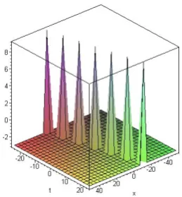
[image:4.595.238.368.439.579.2](3.4)
Figure 1: Graphical representation of solution (3.4), for λ = 4, µ = 2, c2 = 2, c3 =
1, a1 = 1, a2 = 2, c1 = 2 and q(t) = t
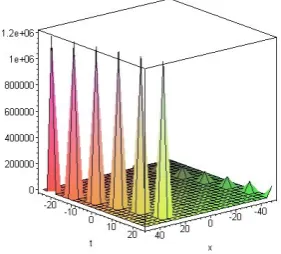
When λ2 −4µ <0, we have trigonometric function solution
u(x, t) = c3 +c2λ
(
1 2
√
(−λ2+4µ)(−a2sin(12((c1x+q(t)) √
(−λ2+4µ)))+a1cos(12((c1x+q(t)) √
(−λ2+4µ)))) (a1sin(12((c1x+q(t))
√
(−λ2+4µ)))+a
2cos(12((c1x+q(t)) √
(−λ2+4µ)))) −
λ 2 ) +c2 ( 1 2 √
(−λ2+4µ)(−a
2sin(12((c1x+q(t)) √
(−λ2+4µ)))+a
1cos(12((c1x+q(t)) √
(−λ2+4µ))))
(a1sin(12((c1x+q(t)) √
(−λ2+4µ)))+a
2cos(12((c1x+q(t)) √
(−λ2+4µ)))) −
Figure 2: Graphical representation of solution (3.5), when λ= 2, µ = 4, c2 = 2, c3 =
1, a1 = 1, a2 = 2, c1 = 2 and q(t) = t
When λ2 −4µ= 0, we get rational solution as follows:
u(x, t) =c3+c2λ
(
A2
A1+A2((c1x+q(t))) −
λ
2
)
+c2
(
A2
A1+A2((c1x+q(t))) −
λ
2
)2
, (3.6)
where A1, A2, a1 and a2 are arbitrary constants.
Figure 3: Graphical representation of solution (3.6), when λ= 2, c2 = 2, c3 = 1, A1 =
1, A2 = 2, c1 = 2 andq(t) =t
5
[image:5.595.238.367.454.588.2]Case 2:
q(t) =q(t), ρ(t) = ρ(t), α0(t) =c3, α1(t) =c2(λ±3
√
−λ2+ 4µ), α
2(t) =c2,
ω(t) = 48ρ(t)c21
c2 , σ(t) =
−156ρ(t)c21
c2 , δ(t) = −(25ρ(t)c
2
1c2λ2−52ρ(t)c21c2µ−24ρ(t)c21λc2(λ±3
√
−λ2+4µ)+48c2 1c3ρ(t))
c2 ,
θ(t) = −(192ρ(t)µc51c3+c2q′(t)+144ρ(t)λ2µc51c2−192ρ(t)µ2c51c2−24ρ(t)λ4c51c2−48ρ(t)λ2c51c3)
c1c2 +−(24ρ(t)λ
3c5 1c2(λ±3
√
−λ2+4µ)−96ρ(t)c5
1c2µλ(λ±3
√
−λ2+4µ))
c1c2 ,
(3.7) where c1, c2 and c3 are arbitrary constants.
Consequently, we have the following three types of exact solutions of (3.1): If λ2−4µ >0, we obtain the hyperbolic function solution in the form
u(x, t) =c3+ (λ±3
√
−λ2+ 4µ)c 2
(
1 2
√
(λ2−4µ)(a
1sinh(Λ1)+a2cosh(Λ1))
(a2sinh(Λ1)+a1cosh(Λ1)) −
λ 2 ) +c2 ( 1 2 √
(λ2−4µ)(a
1sinh(Λ1)+a2cosh(Λ1))
(a2sinh(Λ1)+a1cosh(Λ1)) −
λ
2
)2
.
(3.8)
If λ2−4µ <0, we have trigonometric function solution in the following form:
u(x, t) = c3+ (λ±3
√
−λ2+ 4µ)c 2
(
1 2
√
(−λ2+4µ)(−a
2sin(Λ2)+a1cos(Λ2))
(a1sin(Λ2)+a2cos(Λ2)) −
λ 2 ) +c2 ( 1 2 √
(−λ2+4µ)(−a2sin(Λ2)+a1cos(Λ2))
(Λ2)+a2cos(Λ2)) −
λ
2
)2
.
(3.9)
If λ2−4µ= 0, we get rational solution as follows:
u(x, t) = c3 +c2(λ±3
√
−λ2+ 4µ)
(
A2
A1+A2((c1x+q(t)))−
λ
2
)
+c2
(
A2
A1+A2((c1x+q(t))) −
λ
2
)2
(3.10) whereA1, A2, a1, a2 are arbitrary constants and Λ1 = 12((c1x+q(t))
√
(λ2−4µ)) and
Λ2 = 12((c1x+q(t))
√(
−λ2+ 4µ)).
Case 3:
q(t) = q(t), ρ(t) =ρ(t), α0(t) = c3, α1(t) = c2(λ±
√
(λ2 −4µ)), α
2(t) =c2,
ω(t) = 48ρ(t)c21
c2 , σ(t) =
−156ρ(t)c2 1
c2 , δ(t) = −(−24ρ(t)c
2 1c2λ((λ±
√
(λ2−4µ)))+13ρ(t)c2
1c2λ2−4ρ(t)c12µc2+48c21c3ρ(t))
c2 ,
θ(t) = −(−36ρ(t)λ 4c
2c51+c2q′(t)+216ρ(t)c51c2λ2µ−288ρ(t)c2µ2c51−144ρ(t)λµc51(c2(λ±
√
(λ2−4µ))))
c1c2 +−(288ρ(t)µc
5
1c3−72ρ(t)λ2c51c3+36ρ(t)λ3c51c2(λ±
√
(λ2−4µ)))
c1c2 ,
(3.11) where c1, c2 and c3 are arbitrary constants.
When λ2 −4µ > 0, we derived hyperbolic function solution of Eq. (3.1) in the
u(x, t) =c3+c2(λ±
√
(λ2−4µ))
(
1 2
√
(λ2−4µ)(a
1sinh(Λ1)+a2cosh(Λ1))
(a2sinh(Λ1)+a1cosh(Λ1)) −
λ
2
)
+c2
(
1 2
√
(λ2−4µ)(a
1sinh(Λ1)+a2cosh(Λ1))
(a2sinh(Λ1)+a1cosh(Λ1)) −
λ
2
)2
.
(3.12)
When λ2 −4µ <0, we have trigonometric function solution of Eq. (3.1) as follows:
u(x, t) = c3+c2(λ±
√
(λ2−4µ))
(
1 2
√
(−λ2+4µ)(−a
2sin(Λ2)+a1cos(Λ2))
(a1sin(Λ2)+a2cos(Λ2)) −
λ
2
)
+c2
(
1 2
√
(−λ2+4µ)(−a2sin(Λ2)+a1cos(Λ2))
(a1sin(Λ2)+a2cos(Λ2)) −
λ
2
)2
.
(3.13)
When λ2 −4µ= 0, we get rational solution of Eq. (3.1) as follows:
u(x, t) = c3 +c2(λ±
√
(λ2−4µ))
(
A2
A1+A2((c1x+q(t))) −
λ
2
)
+c2
(
A2
A1+A2((c1x+q(t)))−
λ
2
)2
(3.14) where A1, A2, c1, c2 and c3 are arbitrary constants Λ1 = 12((c1x+q(t))
√
(λ2−4µ))
and Λ2 = 12((c1x+q(t))
√(
−λ2+ 4µ)).
4
Conclusion and Remarks
In this article, we have established certain new solutions of the Shallow water wave equation (3.1) by using generalized (GG′)-expansion method. These solutions are ex-pressed in terms of hyperbolic, trigonometric, and rational functions involving arbi-trary parameters. Also, we have presented graphical representation of solutions (3.4), (3.5) and (3.6) in Figure 1, Figure 2, Figure 3 respectively. In the similar way we can represent graphically the behavior of other derived solutions. It is imperative to state that some of our solutions are expressed in terms of physical parameter q(t) and ρ(t) = t and it plays a crucial role as the remaining coefficients of equation (3.1) have all been expressed in terms of it. In fact, the various other arbitrary constants occurring in the solutions, along withq(t), ρ(t), provide further freedom to simulate the desired physical situations. In almost all the cases the solutions obtained may also help to recover certain solutions available in literature for the particular models with constant coefficients. It is worth to mention here that the correctness of the solutions has been checked with the aid of software MAPLE.
References
[1] M. J. Ablowitz and P. A. Clarkson,Solitons, Nonlinear Evolution Equations and Inverse Scattering Transform, Cambridge University Press, Cambridge, 1991.
[2] R. Hirota, Exact solution of the KdV equation for multiple collisions of solutions,
[3] S. L. Zhang, B. Wu and S. Y. Lou, Painlev´e analysis and special solutions of generalized Broer-Kaup equations, Phys. Lett. A, 300 (2002) 40-48.
[4] M. R. Miura, B¨acklund Transformation, Springer- Verlag, Berlin, 1978.
[5] C. Rogers and W. F. Shadwick, Ba¨cklund Transformations, Academic Press, New York, 1982.
[6] J. H. He and X. H. Wu, Exp-function method for nonlinear wave equations,
Chaos Soliton Fract., 30 (2006) 700-708.
[7] A. Bekir and A. Boz, Exact solutions for nonlinear evolution equations using Exp function method,Phys. Lett. A, 372 (2008) 1619-1625.
[8] S. Zhang, Application of Exp-function method to higher dimensional nonlinear evolution equation, Chaos Soliton Fract., 38 (2008) 270-276.
[9] N. A. Kudryashov, Exact solutions of the generalized Kuramoto-Sivashinsky equation, Phys. Lett. A, 147 (1990) 287-291.
[10] M. A. Abdou, The extended tanh-method and its applications for solving non-linear physical models, Appl. Math.Comput., 190 (2007) 988-996.
[11] L. Wazzan, A modified tanh-coth method for solving the KdV and KdV- Burgers equation, Commu. Nonlinear Sci. Numer. Simul., 14 (2009) 443-450.
[12] D. Lu, Jacobi elliptic function solutions for two variant Boussinesq equations,
Chaos Soliton Fract., 24 (2005) 1373-1385.
[13] S. Liua, Z. Fua, S. Liua and Q. Zhaoa, Jacobi elliptic function expansion method and periodic wave solutions of nonlinear wave equations, Phys. Lett. A, 289 (2001) 6974.
[14] K. Singh, R. K. Gupta and S. Kumar, Benjamin-Bona-Mahony (BBM) equa-tion with variable coefficients: Similarity reducequa-tions and Painlev´eanalysis,Appl. Math. Comput., 217 (2011) 7021-7027.
[15] S. Kumar, K. Singh and R. K. Gupta, Painlev´e analysis, Lie symmetries and exact solutions for (2+1)-dimensional variable coefficients Broer-Kaup equations,
Comm. Nonlinear Sci. Numer. Simulat., 17 (2012) 1529-1541.
[16] L. Kaur and R. K. Gupta, Kawahara equation and modified Kawahara equa-tion with time dependent coefficients: symmetry analysis and generalized (GG′) expansion method, Math. Meth. Appl. Sci., 36 (2013) 584-600.
[17] M. L. Wang, X. Li and J. Zhang, The (GG′)-expansion method and travelling wave solutions of nonlinear evolution equations in mathematical physics, Phys. Lett. A, 372 (2008) 417-423.
[18] S. Zhang, L. Dong, J. M. Ba and Y. N. Sun, The (GG′)-expansion method for nonlinear differential difference equations, Phys. Lett. A, 373 (2009) 905-910.