Analysis, programming and evaluation of calculation methods for Value-at-Risk involving risk-factor models with heavy tails

(1)

MASTER THESIS IN MATHEMATICS /APPLIED MATHEMATICS

Analysis, programming and evaluation of calculation methods for

Value-at-Risk involving risk-factor models with heavy tails

by

Natalia Arango Mesa

Danuwat Weereerat

Magisterarbete i matematik/tillämpad matematik

DIVISION OF APPLIED MATHEMATICS

SCHOOL OF EDUCATION, CULTURE AND COMMUNICATION

MÄLARDALEN UNIVERSITY

(2)

2 Master thesis in mathematics / applied mathematics

Date: 2009-06-05

Project name:

Analysis, programming and evaluation of calculation methods for Value-at-Risk involving risk-factor models with heavy tails

Authors:

Natalia Arango Mesa Danuwat Weereerat

Supervisor: Jan Röman

Examiner:

Anatoliy Malyarenko

(3)

3

1 Abstract

It is known that normal distributions of asset returns is a key assumption made by many financial models, including the capital asset pricing model (CAPM) and the Black-Scholes option pricing model (BSM). However, actual asset returns may not follow this distribution, since the improbability of unlikely market events is overestimated. Empirical studies on financial time series indicate that the distribution of asset returns is often leptokurtic which has a peak around the mean and heavier tail than a normal distribution.

In order to account for this fact, Monte-Carlo and Historical Simulation methods are implemented to calculate Value-at-Risk for a portfolio of an investment in international equity indices, assuming for the risk factors changes the following models:

 Multivariate Normal Distribution

 Multivariate Student’s t Distribution

 t-Copula with non-parametrical marginal distributions – CLM method

 t-Copula with Student’s t marginal distributions – IFM method

 t-Copula applying Extreme Value Theory for the tails – EVT method

 AR(1)-GARCH(1,1)

(4)

4

2

3 Introduction

It is known that normal distributions of asset returns is a key assumption made by many financial models, including the capital asset pricing model (CAPM) and the Black-Scholes option pricing model (BSM). However, actual asset returns may not be so normal, because the improbability of unlikely market events is overestimated.

Using a normal distribution, events that diverge from the mean by five or more standard deviations are very rare and events that diverge from the mean by ten or more standard deviations are even more uncommon. However, events deemed nearly impossible by models assuming normal asset return distributions are possible in the financial markets and do occur.

The statistical irregularities, in which very low and high values are more frequent than what a normal distribution predicts, are known as heavy tails. In a normal distribution, the tails to the extreme left and extreme right of the mean become smaller, ultimately reaching zero occurrences. However, some real life statistical series demonstrate occurrences of low and high values that are greater than theoretically expected by a normal distribution.

(6)

6

4 Theoretical background

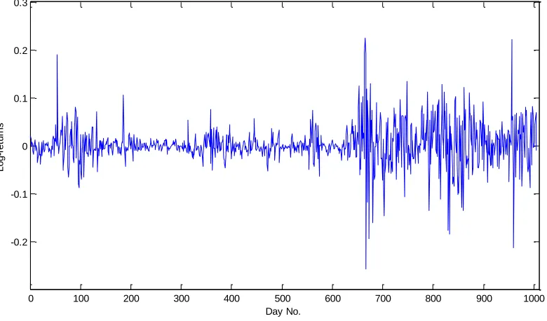
Empirical studies on financial time series indicate that the distribution of asset returns is often leptokurtic which has a peak around the mean and heavier tail than a normal distribution (Cont 2001). To illustrate further, the tail behavior of the asset returns may be investigated from the iTraxx credit default swap index1. The sample of daily data covers the period 05/01/2005 – 21/11/2008.

Figure 4-a: Log returns of iTraxx index from period 05/01/2005 - 21/11/2008

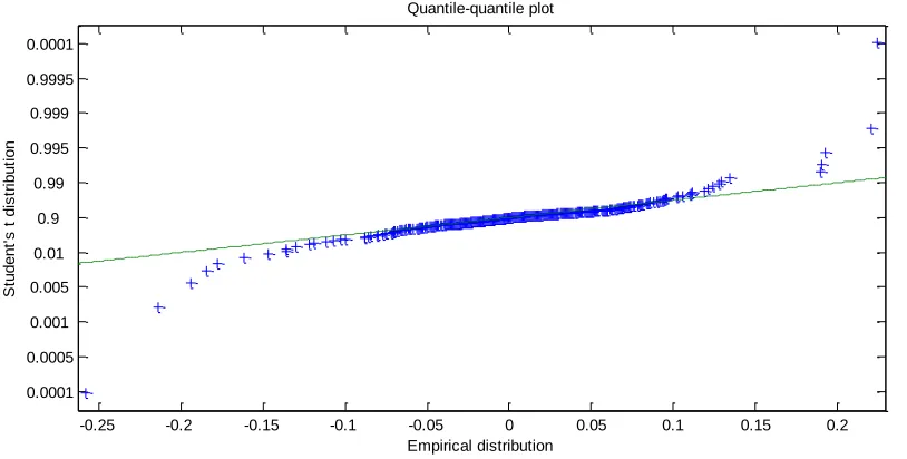
Figure 4-b and Figure 4-c show the quantile-quantile plot for the fitted normal distribution and Student’s t distribution, respectively. It can be observed that the normal distribution does not fit the data; especially for both the negative and positive tails. On the other hand, Student’s t distribution can capture the tails behavior and fit more accurately.

1

http://www.indexco.com

0 100 200 300 400 500 600 700 800 900 1000

-0.2 -0.1 0 0.1 0.2 0.3

Day No.

L

o

g

-r

e

tu

rn

(7)

7

Figure 4-b: Quantile-quantile plot for the normal distribution with parameters estimated from the daily returns of iTraxx index.

Figure 4-c: Quantile-quantile plot for the Student’s t distribution with parameters estimated from the daily returns of iTraxx index

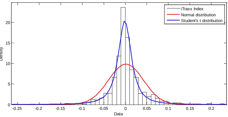
Since the previous analysis shows that the data is not normally distributed, a Student’s t distribution is used in order to reproduce the model; its parameters are estimated from the log likelihood function as explained on section 5.2. The result suggests that the returns of the iTraxx index have heavier tail and kurtosis significantly greater than the normal model.

The probability density functions for the distributions fitted as well as a histogram of the historical data are shown in Figure 4-d.

(8)

8

Figure 4-d: Probability density functions for the distribution fitted to the iTraxx index

In order to take into account this reality, Monte-Carlo and Historical Simulation methods are implemented to calculate Value-at-Risk (VaR) for a portfolio. The following models for the risk-factor changes are assumed for a portfolio of an investment in international equity indices:

 Multivariate Normal Distribution: VaR is calculated by using the standard Monte Carlo simulation method and assuming a multivariate normal distribution for the risk-factor changes.

 Multivariate Student’s t Distribution: The standard Monte Carlo simulation method is also used but a multivariate Student’s t distribution is used to model the risk-factor changes. The parameters are estimated by the maximum likelihood method.

 t-Copula with non-parametrical marginal distributions – CLM method: The Monte Carlo simulation method is performed assuming that the risk factors follow a t-Copula distribution with nonparametric marginal distributions.

 t-Copula with Student’s t marginal distributions – IFM method: Similar to the previous method but the marginal distributions are fitted with the Student’s t distribution.

 t-Copula applying Extreme Value Theory for the tails – EVT method: The tails of the distributions are modeled by a generalized Pareto distribution (GPD) and the body is modeled by an empirical distribution.

 AR(1)-GARCH(1,1): A conditional historical simulation method in which AR(1)-GARCH(1,1) model with Student’s t innovation are fitted to the historical data. Bootstrapping is performed to draw with replacement from the series of the standardized residuals. The standardized residuals are used to simulate the risk-factor changes.

The calculations results are tested by using the so-called backtesting method. An Unconditional Coverage Test and an Independence test are applied in order to evaluated and compare the goodness of the models.

-0.25 -0.2 -0.15 -0.1 -0.05 0 0.05 0.1 0.15 0.2 0

5 10 15 20

Data

D

e

n

s

it

y

(9)

9

5 Risk-Factor Models

This section provides several different models for the risk-factor changes. These models can be implemented with Monte Carlo or Historical simulation to estimate the loss of a portfolio as explained in section 6.2.

5.1 Multivariate Normal Distribution

The risk-factor changes 𝑿 = (𝑋1, … , 𝑋𝑛)′ are assumed to come from a multivariate normal distribution,

𝑿 = 𝝁 + 𝐴𝒁

Where𝒁 = (𝑍1, … , 𝑍𝑘)′ is a vector of i.i.d. univariate standard normal random variables (i.e., with mean zero and variance one), and 𝐴 ∈ ℝ𝑛∗𝑘 and 𝝁 ∈ ℝ𝑛 are a matrix and a vector of constants. It is readily shown than 𝐸 𝑿 = 𝝁 and 𝑐𝑜𝑣 𝑿 = 𝛴 where 𝛴 = 𝐴𝐴′

5.1.1 Simulation

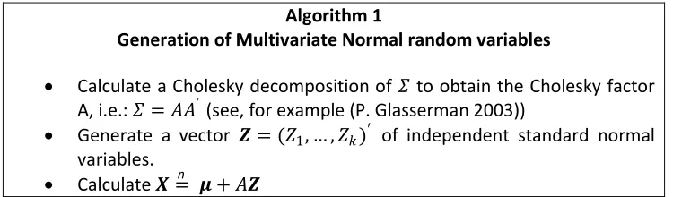
In order to generate the path 𝑋 _𝑡+1(1), … , 𝑋 _𝑡+1(𝑘) three steps are followed:

Algorithm 1

Generation of Multivariate Normal random variables

 Calculate a Cholesky decomposition of 𝛴 to obtain the Cholesky factor A, i.e.: 𝛴 = 𝐴𝐴′ (see, for example (P. Glasserman 2003))

 Generate a vector 𝒁 = (𝑍1, … , 𝑍𝑘)′ of independent standard normal variables.

 Calculate 𝑿 = 𝝁 + 𝐴𝒁

To illustrate the performance, the parameters 𝜇 and 𝐴 are estimated for the daily returns of a portfolio of an investment in five international equity indices. The MSCI indices2 representing the global stock market indices for the period 01/01/2008 to 31/12/2008 are used. The portfolio is compose of 12.5% of USA index (NDDUUS), 12.5% of Europe index (NDDUE15), 12.5% of EM index (NDUEEGF), 12.5 of Asia excluding Japan (NDUECAXJ) and 50% of Sweden index (NDDLSW).

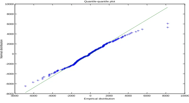
Figure 5-a shows the quantile-quantile plot for the fitted normal distribution. It is observed that the normal model is a good approximation for small returns, but for both the negative and positive tails the distribution does not fit the data.

2

Equity market performance of the developed markets in Europe (http://www.mscibarra.com).

n

(10)

10

Figure 5-a: Quantile-quantile plot for the normal distribution with parameters estimated from the daily returns of a portfolio of an investment in five international equity indices.

5.2 Multivariate Student’s t Distribution

The variable 𝑿 = 𝜇 + 𝑊𝐴𝒁is said to have a (multivariate) normal variance mixture distribution where

(i) 𝒁~𝑁𝑘(𝟎, 𝑰𝑘) represents 𝑘 i.d.d. multivariate standard normal random variables,

(ii) 𝑊 ≥ 0 is a scalar random variable independent of 𝒁and

(iii) 𝐴 ∈ ℝ𝑛∗𝑘 and 𝜇 ∈ ℝ𝑛 are a matrix and a vector of constants.

If 𝑊~𝐼𝑛𝑣 − 𝐺𝑎𝑚𝑚𝑎 1₂𝑣,1₂𝑣 , i.e. 𝑊 follows an inverse gamma distribution with shape parameter 1₂𝑣

and scale parameter1₂𝑣, then 𝑊/𝑣~𝐼𝑛𝑣 − 𝑐𝑕𝑖 − 𝑠𝑞𝑢𝑎𝑟𝑒(𝑣) (which is equivalent to saying that _𝑊𝜈 ~𝜒𝑣2) and therefore 𝑿has a multivariate t distribution with 𝑣 degrees of freedom:

𝑿~𝑡𝑛(𝑣, 𝝁, 𝜮)

where 𝛤 represents the gamma function, 𝛴 represents the covariance matrix, 𝛴

1

2_{is the square root of}

the determinant of 𝛴 and 𝑛 is the number of risk factors.

(11)

11 5.2.1 Parameters estimation

Under multivariate Student’s t distribution, the most asymptotically efficient estimator of the parameters is the solution of maximizing the log-likelihood function based on its density (Kan and Zhou 2006),

Since the function does not allow the explicit solution for its maximum, the EM algorithm (see (Kan and Zhou 2006)) is used in order to obtain explicit iterative formulas to find the parameters estimate that maximizes the log-likelihood function under 𝑡, i.e., the solution to maximizing ℒ.

Starting from an initial estimate for 𝜇 and 𝛴: 𝜇 (1)= 𝜇 , 𝛴 (1)= 𝛴 =𝑣−2_𝑣 𝑉 , the iterative estimates are

where 𝑢𝑡(𝑖) is an auxiliary variable whose meaning as well as why the algorithm works can be found in the reference (Kan and Zhou 2006) and is derived as follows.

5.2.1.1 EM Algorithm

As explained before, a t distribution is an infinite mixture of the normals, therefore there exists

𝑢𝑡~𝜒𝑣2/𝑣 such that, conditional on 𝑢𝑡, 𝑥𝑡~𝑁(𝜇,_𝑢𝛴

𝑡) and has the conditional log-likelihood function

ℒ 𝑥_𝑡 𝑢𝑡 =

which can be maximized with

(12)

12

𝐸 𝑢_𝑡|𝑥_𝑡; 𝜇, 𝛴 = 𝑣 + 𝑛

𝑣 + 𝑥_𝑡− 𝜇 ′_𝛴−1_𝑥

𝑡− 𝜇

This estimate is calculated for any initial estimate of the parameters 𝜇 and 𝛴. The M-step consists then on maximizing the conditional log-likelihood function. The maximization updates the most recent value of the parameter estimates which can be used in turn to update a new estimate for 𝑢𝑡, therefore, by implementing repeated iterations the solution converges to the value that maximizes the unconditional log-likelihood function.

The procedure is then implemented as follows

Algorithm 2

Parameters estimation for the Multivariate Student’s t distribution

 Define the initial estimates for 𝜇 and 𝛴

 Calculate the log-likelihood function based on the parameters

estimated until the solution converges to the value that maximizes the function.

5.2.1.2 Estimation of the Degrees of Freedom

The algorithm considers the degrees of freedom 𝑣 to be known. When 𝑣 is unknown it can be treated as an additional parameter and estimated from the data as explained below

Algorithm 3

Estimation of the degrees of freedom

(13)

13 5.2.2 Simulation

Once the parameters 𝜇, 𝛴 and 𝑣 are obtained, the following steps are followed in order to generate a path of multivariate t-distributed random variables

Algorithm 4

Generation of Multivariate Student’s t random variables

 Calculate a Cholesky decomposition of 𝛴 to obtain the Cholesky factor A, i.e.: 𝛴 = 𝐴𝐴′ (see, for example (P. Glasserman 2003))

 The multivariate Student’s t random variables can be obtained then as

𝑿 𝜇 + 𝑊𝐴𝒁𝑛

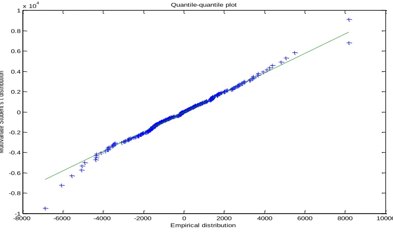
The advantage of the multivariate Student’s t model over the previous normal model is that, as illustrated by the quantile-quantile plot in Figure 5-b, the tails of the empirical distribution can be reproduced more accurately.

Figure 5-b: Quantile-quantile plot for the multivariate-t distribution with parameters estimated from the daily returns of a portfolio of an investment in five international equity indices.

(14)

14

5.3 Copulas

Copulas have become widely used in practice to model a multivariate distribution. It is an alternative way to model the dependence between risk factors. To understand the concept of copula, it is necessary to illustrate first the idea of marginal distributions and transformation.

Let 𝑋 be a random variable with the cumulative distribution function 𝐹. 𝐹−1represents the inverse cumulative distribution function (quantile function), i.e.

𝐹−1_{𝑝 = 𝑖𝑛𝑓 𝑥 ∈ 𝑅: 𝑝 ≤ 𝐹(𝑥)}_{, for a probability}_{0 < 𝑝 < 1}_.

Then

1. For any uniformly distributed variable 𝑈~𝑈(0,1) it is possible to simulate random variables with the distribution function 𝐹 by having 𝐹−1(𝑈)

2. If 𝐹 is continuous then 𝐹(𝑋) is a standard uniform distributed variable, i.e. 𝐹(𝑋)~𝑈(0,1). This method can be used to transform any random variable to a uniform distribution.

In probability theory, given the joint distribution of two events 𝑋 and 𝑌, the marginal distribution 𝑃(𝑋) of the event 𝑋 is the unconditional probability of 𝑋, i.e. the probability distribution of 𝑋 regardless of event Y occurring. The marginal distribution function is computed by summing the joint probability over the other variable (in this, variable 𝑌). In the continuous case, it is obtained by integration.

When modeling a multivariate distribution, the most important factor is to model the dependence of the random variables. The dependence among the random variable 𝑋1, … , 𝑋𝑛 is described by their joint distribution function.

𝐹 𝑥1, . . , 𝑥𝑛 = 𝑃 𝑋1≤ 𝑥1, … , 𝑋𝑛 ≤ 𝑥𝑛

The random vector 𝑥 may be transformed in order to obtain a set of standard uniform distributed variable, 𝑈(0,1), by using the marginal cdf of 𝑿. Assuming that the marginal distributions of the random variable 𝑋1, . . , 𝑋𝑛 are 𝐹1, . . , 𝐹𝑛 the transformation is expressed as

𝑥1, . . , 𝑥𝑛 𝑇↦ 𝐹1(𝑥1), . . , 𝐹𝑛(𝑥𝑛) 𝑇

The joint distribution function 𝐶 of 𝐹1(𝑋1), . . , 𝐹𝑛(𝑋𝑛) 𝑡 is called the copula of the random variable 𝑋1, . . , 𝑋𝑛 𝑇, i.e.

𝐹 𝑥₁, . . , 𝑥_𝑛 = 𝑃 𝐹1(𝑋1) ≤ 𝐹1(𝑥1), … , 𝐹𝑛(𝑋𝑛) ≤ 𝐹𝑛(𝑥𝑛) = 𝐶 𝐹1(𝑥1), … , 𝐹𝑛(𝑥𝑛)

Sklar’s Theorem

(15)

15

Sklar’s theorem implies that all multivariate distribution functions contain a copula and that the copula could be used in conjunction with arbitrary margins in order to construct the multivariate distribution function. For example, building a distribution with the Student’s t copula but arbitrary margins such as univariate Student’s t, exponential distribution, etc. is known as a meta-tv distribution, where the Student’s t copula is used to combine the margins together.

The multivariate Student’s t copula

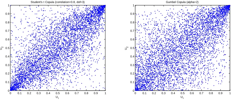
There are a number of copulas such as Gaussian (normal) copula, Gumbel copula, Student’s t copula, etc. This paper focuses on the Student’s t copula by assuming that the risk-factor changes follow the Student’s t copula. Student’s t copula is often used in financial applications because of its properties. The advantage of the t-Copula is that it can capture the lower and upper tail dependence as demonstrated by Figure 5-c. When extreme events occur, the risk-factors tend to be highly correlated. Therefore, it is often used in risk management as it allows for modeling these joint extreme co-movements.

Figure 5-c: Five thousand simulated points from Student's t copula and Gumbel copula

A 𝑛-dimensional copula is basically a multivariate cumulative distribution function with uniform distributed margins in [0,1]. The copula of the multivariate standardized Student’s t distribution is the Student’s t copula and is defined as

(16)

16

𝐶 𝑢₁, … , 𝑢_𝑛; 𝛴, 𝑣 = 𝑇_𝛴,𝑣(𝑡_𝑣−1_𝑢

1 , … , 𝑡𝑣−1 𝑢 𝑛 )

where 𝑇𝛴,𝑣 is the standardized multivariate Student’s t distribution function, 𝛴 is the correlation matrix,

𝑣 are the degrees of freedom and 𝑡𝑣−1 𝑢 denotes the inverse of the Student’s t cumulative distribution function.

5.3.1 Rank Correlation

The most common dependence measure used is linear correlation. It plays a central role in multivariate normal distribution. However, (Embrechis, McNeil and Straumann 1999) presents several shortcomings:

- The variances of 𝑋 and 𝑌 must be finite for the correlation to exist.

- The independence of two random variables implies that they are uncorrelated but the converse is true only for a multivariate normal distribution.

- Linear correlation is not invariant under non-linear increasing transformations. So that the transformation does not preserve linear correlations, however, preserve rank correlations. The correlation between the variables is then captured by calculating rank correlation. Rank correlations are simple measures of dependence that depend only on the copula of a bivariate distribution. It can be used to fit a copula to the empirical data. There are two main types of rank correlation, Kendall’s tau and Spearman’s rho. The Kendall’s tau will be discussed here.

5.3.1.1 Kendall’s tau

Kendall’s tau can be interpreted as a measure of concordance for bivariate random variable whereas linear correlation measures the degree of linear dependence only. Denote a random sample of 𝑛 observations 𝑋1, 𝑌1 , … , 𝑋𝑛, 𝑌𝑛 from a vector (𝑋, 𝑌) of continuous random variables. There are distinct pairs 𝑋𝑖, 𝑌𝑖 and 𝑋𝑗, 𝑌𝑗 of observations in the sample, and each pair is either concordant (i.e.,

𝑋𝑖 < 𝑌𝑖 and 𝑌𝑖 < 𝑌𝑗, or 𝑋𝑖 > 𝑋𝑗 and 𝑌𝑖 > 𝑌𝑗) or discordant (i.e., 𝑋𝑖 < 𝑌𝑖 and 𝑌𝑖 > 𝑌𝑗, or 𝑋𝑖 > 𝑋𝑗 and

𝑌_𝑖 < 𝑌_𝑗); if we call 𝑐 the number of concordant pairs, and 𝑑 the number of discordant pairs, then an

estimate of Kendall’s rank correlation for the sample is given by

𝜏 = 𝑐 − 𝑑

c + d

In higher dimensions the Kendall’s tau matrix is analogous to the linear correlation, where the Kendall’s tau matrix has 𝑛 × 𝑛 pairwise correlation.

For elliptical distribution3, Kendall’s tau matrix 𝜏(𝑈) could be transform to the correlation matrix Σ by:

3_{Elliptical distributions are generalizations of the multivariate normal distribution. The contour lines of the}

distribution have an elliptical shape. The random matrix 𝑿 has a multivariate elliptical distribution, 𝑿~𝐸𝑛 𝝁, 𝚺, 𝜓 ,

if its characteristic function can be defined as

𝜙𝑋 𝒕 = 𝑒 𝑖𝒕𝑇𝝁 𝜓 𝒕𝑇𝚺𝐭

(17)

17

Σ_𝑥,𝑦 = sin 𝜋𝜏 𝑥, 𝑦

2

See (Lindskog, Mcneil and Schmock 2002) for proof. However, it could happen that this transformation of matrix of Kendall’s rank correlation will not give a positive definite correlation matrix. In this case, Σ can be transform by the eigenvalue method. The Kendall’s tau might be applied to parameter estimation of t-Copula. The remaining parameter 𝜈 of the t-Copula could then be estimated by maximum likelihood, as discussed later in section 5.3.2.

Algorithm 5 The Eigenvalue Method

 Decompose correlation matrix Σ = Λ𝐷Λ−1

where D is a diagonal matrix formed from the eigenvalue of Σ

Λ is an orthogonal matrix whose columns are the corresponding eigenvector of Σ

 Replace all negative eigenvalues in D by small value 𝛿 > 0 to recieve diagonal matrix 𝐷

 Compute Σ = Λ𝐷 Λ−1which will be symmetric positive definite matrix

5.3.2 Parameters estimation

Assume that the empirical data are time series 𝑿 = 𝒙1𝑡, … , 𝒙𝑛𝑡 𝑇, 𝑡 = 1, … , 𝑇 where n represents the number of risk factors and 𝑇 represents the number of observations. The empirical data might be the following observation matrix:

𝑿 =

𝑥₁₁ ⋯ 𝑥_1𝑇

⋮ ⋱ ⋮

𝑥_𝑛1 ⋯ 𝑥_𝑛𝑇

Additionally, it is assumed that the joint distribution function 𝐹 has continuous marginal distribution 𝐹1, … , 𝐹𝑛. By Sklar’s theorem, there exists a unique copula satisfying

𝐹 𝑥 = 𝐶 𝐹₁(𝑥₁), … , 𝐹_𝑛(𝑥_𝑛) . The parameters of the copula are estimated by maximum likelihood

method. In practice, the marginal distributions have to be estimated as well in order to estimate the copula. A number of appropriate models might be chosen, for example, the generalized hyperbolic distribution, or its special cases such as Normal inverse Gaussian or Student’s t distribution which will be discussed later. Since the copula data are seldom observed directly, the estimation marginal distribution and the copula are split into two steps:

- Estimating marginal distributions and forming a pseudo sample - Calibrating the copula from a pseudo sample

5.3.2.1 Estimating marginal distributions

(18)

18 Parametric estimation (IFM method)

The Inference Functions for Margins (IFM) method indicates that the parameters of the marginal distributions are estimated separately from the parameters of the copula. The appropriate marginal distribution is chosen to fit by Maximum Likelihood method:

𝛼 _𝑖 = 𝑎𝑟𝑔𝑚𝑎𝑥ℒ𝑖_(𝛼

Student’s t distribution is well used in financial models especially in the field of risk management, due to its heavy tails. With the aid of copula, it is possible to construct the Student’s t distribution with

Parameters 𝜇, 𝜎 and 𝜈 could be estimated by maximize log-likelihood function:

ln ℒ𝑖_{𝜇 , 𝜎 , 𝜈 = ln 𝑓}

𝑖 𝑥𝑖1, … , 𝑥𝑖𝑇; 𝜇 , 𝜎 , 𝜈 = ln 𝑓𝑖 𝑥𝑖𝑡; 𝜇 , 𝜎 , 𝜈

𝑇

𝑡=1

In fact, this function could be transformed to unconstrained optimization problem which is much easier to solve.

ln ℒ𝑖_{𝜇 , 𝜎 , 𝜈 = ln 𝑓}

𝑖 𝑥𝑖𝑡; 𝜇 , 𝜎 , 𝜈

𝑇

𝑡=1

The following initial values of parameters might be used.

(19)

19 where 𝑚𝑘= 𝑥𝑖𝑡−𝜇 _𝑇 0

𝑘 𝑇

𝑡=1

Non-parametric estimation (CML method)

The Canonical Maximum Likelihood (CML) method differs from the IFL method because no assumptions are made about the parametric form of the marginal distributions. The empirical distribution function

𝐹_𝑖could be estimated by:

𝐹 _𝑖 𝑥 =_{𝑇 + 1}1 1 𝑥_𝑖𝑡 ≤ 𝑥

𝑇

𝑡=1

The factor _𝑇+11 is used to make sure 𝐹 𝑖 𝑥 ∈ [0,1). Evaluation of distribution functions at the boundary 1 might cause a problem. The empirical distribution may be computed by finding the ranks of observation data. It is simpler and saves calculation time. The empirical distribution is just𝑟𝑎𝑛𝑘 (𝑥_𝑁+1𝑖𝑡). The implementation of this method is the following:

- Set a marker for remembering the original of each empirical data set 𝑥𝑖𝑡, 𝑖 = 1, … , 𝑛 and

𝑡 = 1, … , 𝑇

𝑥_𝑖1 ⋯ 𝑥_𝑖𝑇

1 ⋯ 𝑇

- Sort 𝑥𝑖𝑡 in ascending

𝑥𝑖𝑗 ⋯ 𝑥𝑖𝑘

𝑗 ⋯ 𝑘

where 𝑥𝑖𝑗 is the lowest value element 𝑥𝑖𝑘 is the highest element - Compute empirical distribution 𝑟𝑎𝑛𝑘 (𝑥_𝑁+1𝑖𝑡)

𝑥_𝑖𝑗 ⋯ 𝑥_𝑖𝑘

𝑗 ⋯ 𝑘

1

𝑇 + 1 ⋯

𝑇 𝑇 + 1

- Set 𝑥𝑖𝑗 back to the original order by sorting a marker

𝑥_𝑖1 ⋯ 𝑥_𝑖𝑇

1 ⋯ 𝑇

𝐹 _𝑖 𝑥𝑖1 ⋯ 𝐹 𝑖 𝑥𝑖𝑇

Extreme value theory for the tails

(20)

20 Threshold exceedances

Threshold exceedances are focused on the behavior of an extreme value which exceeds a predefined variable (high threshold). Let 𝑿 = 𝒙1, … , 𝒙𝑇 ,𝑇 be a time series observations, an excess over a threshold 𝑢 is defined by 𝑦 = 𝑥𝑡− 𝑢 when 𝑥𝑡 > 𝑢 for any 𝑡 = 1, … , 𝑇. The excess distribution over the threshold 𝑢 has the density function:

𝐹𝑢 𝑦 = 𝑃 𝑋 − 𝑢 ≤ 𝑦|𝑋 > 𝑢 = distribution (GPD) is defined as:

𝐺𝜉,𝜎,𝜐 𝑥 = 1 − 1 + 𝜉

There are several methods of fitting a GPD. A commonly used method is the maximum likelihood. Given observations 𝑥1, … , 𝑥𝑇, a random number 𝑁𝑢 will exceed the high threshold 𝑢. For each of these

The remaining problem is only how to determine a high threshold 𝑢. If a value of 𝑢 is too large, there will be few exceedances and consequently imprecise tail estimators. On the other hand, a value of 𝑢 too small yields too biased tail estimators. The appropriate high threshold can be implicitly detected from plot of the empirical mean excess function:

𝑢, 𝑒_𝑛 𝑢

(21)

21

If the GPD model holds, this plot should become increasingly linear for higher value of 𝑢. Tail probability

In general, the GPD model for excess loss is used to estimate the tail distribution. Furthermore, the tail distribution may be combined with a body estimated from the empirical distribution. The tail distribution might be represented by:

𝐹 𝑥 = 1 − 𝐹 𝑢 𝐹𝑢 𝑥 − 𝑢 + 𝐹 𝑢

After determining a high threshold 𝑢 and the parameters of the GPD model, 𝐹 𝑢 could be computed by the simple empirical estimator𝑇−𝑁_𝑇 𝑢. As a result, the tail probability is obtained by:

𝐹 𝑥 = 1 −𝑁𝑢

𝑇 1 + 𝜉

𝑥 − 𝑢 𝜎

−1/𝜉

The inverse function for a given probability 𝑞 > 𝐹 𝑢 is simply obtained as:

𝐹 −1_{𝑞 = 𝑢 +}𝜎 from the estimated model as data. The GPD tail distribution and empirical distribution for the body is applied to the marginal to form a pseudo sample from residuals. In particular, the marginal 𝐹𝑖 , 𝑖 =

(22)

22 Finally, the simulated risk factor is obtained from

𝑥_𝑡+1𝑖 _{= 𝜇}

𝑡+1𝑖 + 𝜎𝑡+1𝑖 𝑞𝑖 𝑍

The performance of this model is tested by implementing EGARCH model as demonstrated in the backtesting section.

5.3.2.2 Calibrating the copula

Let 𝐹1, … , 𝐹𝑛 be estimated marginal cumulative distribution functions from the above section. The

pseudo-sample from the copula is the following matrix

𝑼 =

Let 𝑐𝜃be a parametric copula density function where θ is the vector of parameters to be estimated. The parameters of the copula are obtained by maximizing the likelihood function:

ln ℒ𝑖_{𝜃 = ln 𝑐}

The copula density function 𝑐𝜃is given by

𝑐_𝜃 𝑢₁, … , 𝑢_𝑛 = 𝑓 𝐹1

−1_𝑢

1 , … , 𝐹𝑛−1 𝑢𝑛

𝑓1 𝐹1−1 𝑢1 … 𝑓𝑛 𝐹𝑛−1 𝑢𝑛

where 𝑓 is the joint density function, 𝑓1, … , 𝑓𝑛 are the marginal density functions and 𝐹1−1, … , 𝐹𝑛−1are the inverse cumulative distribution functions.

For Student’s t copula, there are two parameters to be estimated, the degrees of freedom (𝜈) and the correlation matrix (𝛴). The density is given by

𝑐_𝜈,𝛴 𝑢₁, … , 𝑢_𝑛 = 𝛴 −12 𝛤

(23)

23

Algorithm 6

Parameter estimation for the Student’s t copula

 Estimate parameter of marginal distribution 𝐹𝑖 , 𝑖 = 1, … , 𝑛 - Parametric model (IFM)

- Nonparametric model (CML) - Extreme Value Theory (EVT)

 Forming a pseudo sample by applying 𝐹𝑖 , 𝑖 = 1, … , 𝑛 to empirical data to obtain matrix 𝑼.

 Compute Kendall’s tau rank correlation 𝜏 𝑼 of a pseudo sample.

 Transform to correlation matrix Σ by Σ = sin 𝜋𝜏 𝑼 ₂ .

 If the correlation matrix is not positive definite, use eigenvalue method

 Maximize the log-likelihood function

ln ℒ𝑖_{𝜃 = ln 𝑐}

𝜈 𝑢1𝑡, … , 𝑢𝑛𝑡

𝑇

𝑡=1

Similar to the multivariate-t, t-Copula model with nonparametric marginal distribution reproduces accurately the tails of the empirical distribution, additionally outperforming the results obtained before, as illustrated by the quantile-quantile plot in Figure 5-d. The advantage is obtained by using a nonparametric model for the marginal distributions, because it does not rely on specific assumptions about the shape of these densities.

Figure 5-d: Quantile-quantile plot for the t-Copula with non-parametric marginal distributions with parameters estimated from the daily returns of a portfolio of an investment in five international equity indices.

5.3.3 Simulation

The attention is directed to Student’s t copula, which belongs to the group of elliptical copulas, because it is widely used in risk factor models. Although there is no explicit form for this copula, the simulation is

(24)

24

simple. The following algorithm is provided in order to generate uniform random variables from the Student’s t copula 𝑢 1, … , 𝑢 𝑛 ~𝑐𝜈,Σ𝑡𝜈 .

Algorithm 7

Simulation of the Student’s t copula

 Find the Cholesky decomposition of 𝐴 of Σ.

 Simulate n standard normal distributed random variable

𝒛 = 𝑧1, … , 𝑧𝑛 𝑇 ~ 𝑁 0,1 .

 Simulate a random variable 𝑠~𝜒𝜈2.

 Set 𝒚 = 𝐴𝒛.

 Set 𝒙 = 𝜈_𝑠𝒚.

 Apply 𝑡𝜈 to each component of 𝒙 and obtain

𝒖 = 𝑢 ₁, … , 𝑢 _𝑛 𝑇 _{= 𝑡}

𝜈 𝑥1 , … , 𝑡𝜈 𝑥𝑛 𝑇

where 𝑡𝜈 denotes the univariate Student’s t cumulative density distribution function

Then, the inverse functions of the estimated marginal distributions are applied to the vector 𝒖 in order to obtain the simulation outcome

𝑥 ₁, … , 𝑥 _𝑛 𝑇 _{= 𝐹}

1−1 𝑢 1 , … , 𝐹𝑛−1 𝑢 𝑛

𝑇

The following relation must hold:

𝐹_𝑖−1_𝑢

𝑖𝑡 = 𝑥𝑖𝑡 for 𝑖 = 1, … , 𝑛 and 𝑡 = 1, … , 𝑇

This will cause an inconvenience for the nonparametric distribution since its inverse distribution function is not continuous. The simulated uniform random variable 𝑢 1, … , 𝑢 𝑛 𝑇will not match the pseudo sample from the empirical data 𝑢1, … , 𝑢𝑛 𝑇. Thus, the interpolation can be applied. It is assumed that the empirical data is large enough so that the error can be ignored.

5.3.4 Example

The following example is presented in order to illustrate the impact of the model when the dependence among asset returns is modeled by t-Copula. In practice, it is difficult to investigate this impact because of the error of the model fitting and the number of samples. Thus, a sample will be simulated instead. In order to reduce the error of model fitting, a large sample of data is used.

(25)

25 - Normal distribution

- Multivariate Student’s t distribution

- Student’s t Copula with nonparametric marginal - Student’s t Copula with t distributed marginal

The results from 10 million simulations are given in the table below

Model 𝑽𝒂𝑹 4

𝟎.𝟗𝟗

𝑽𝒂𝑹 − 𝑽𝒂𝑹

𝑽𝒂𝑹 𝑽𝒂𝑹 𝟎.𝟗𝟓

𝑽𝒂𝑹 − 𝑽𝒂𝑹 𝑽𝒂𝑹

t-Copula with t-marginal 6.1939 0.4456% 3.5800 0.2151%

t-Copula with non-parametric 6.1940 0.4459% 3.5816 0.2612%

Multivariate normal 5.4428 11.7361% 3.8453 7.6425%

Multivariate Student’s t 5.8753 4.7219% 3.4966 2.1192%

As expected, the assumption of normal distribution gives an under-estimated VaR, with a deviation of more than 11% for the 99% estimate. Multivariate Student’s t distribution performs better under fat tailed data; however, it cannot capture the tail dependence. It is interesting to note that t-Copula with non-parametric marginal gives an estimate very close to the Student’s t marginal’s assumption.

4_𝑉𝑎𝑅

(26)

26

6 Value-at-Risk

Value-at-Risk (VaR) is widely used in risk management. VaR is a method of assessing risk that uses standard statistical techniques routinely used in other technical fields. It measures the worst expected loss over a given horizon under normal market conditions at a given confidence level (Jorion 2001). Risk factors model, as discussed earlier, could be implemented to compute VaR.

6.1 Definition of Value-at-Risk

Given some confidence level 𝛼 ∈ (0, 1), the VaR of a portfolio at the confidence level 𝛼 is given by the smallest number 𝑙 such that the probability that the loss 𝐿 exceeds 𝑙 is no larger than (1 − 𝛼)(McNeil, Frey and Embrechts 2005). Mathematically it is defined as

𝑉𝑎𝑅𝛼 = 𝑖𝑛𝑓 𝑙 ∈ ℝ: 𝑃 𝐿 > 𝑙 ≤ 1 − 𝛼 = 𝑖𝑛𝑓 𝑙 ∈ ℝ: 𝐹𝐿(𝑙) ≥ 𝛼

where

𝐹_𝐿 𝑙 = 𝑃 𝐿 ≤ 𝑙

6.2 Calculation methods

There are several approaches to calculating or approximating loss probabilities and VaR, each representing a tradeoff between accuracy and tractability. The selection decision often relies on the complexity of the portfolio and on the accuracy required. Some standard methods used in the financial industry and implemented trough the paper are introduced.

6.2.1 Variance-Covariance method

Denote 𝑉(𝑡) as the portfolio value, for a given time horizon ∆ the loss of the portfolio over a period

[𝑠, 𝑠 + ∆] is

𝐿_{[𝑠,𝑠+∆]}= − 𝑉 𝑠 + ∆ − 𝑉(𝑠) and 𝐿_𝑡+1 = − 𝑉_𝑡+1− 𝑉_𝑡

The portfolio value can be represented as a function of time and a 𝑛-dimensional random vector

𝑍_𝑡 = (𝑍_𝑡1_{, … , 𝑍}

𝑡𝑛) of risk factors, this is 𝑉𝑡 = 𝑓(𝑡, 𝑍𝑡). The risk factor changes (𝑋𝑡) are then defined as

𝑋_𝑡 = 𝑍_𝑡−𝑍𝑡−1 and the portfolio loss can be written as

𝐿_𝑡+1= − 𝑓(𝑡 + 1, 𝑍_𝑡+ 𝑋_𝑡+1) − 𝑓(𝑡, 𝑍_𝑡)

The loss operator 𝑙[𝑡] which maps risk-factors into losses is then defined as

𝑙_𝑡 𝑥 = − 𝑓 𝑡 + 1, 𝑍𝑡+ 𝑥 – 𝑓 𝑡, 𝑍𝑡 and 𝐿𝑡+1= 𝑙 𝑡 (𝑋𝑡+1).

Assuming that 𝑓 is differentiable it is obtained the first order approximation 𝐿∆𝑡+1= − 𝑓𝑡(𝑡, 𝑍𝑡) +

𝑓_𝑧_𝑖

𝑛

𝑖=1 (𝑡, 𝑍𝑡)𝑋𝑡+1,𝑖 , where the subscripts of 𝑓 denote partial derivatives. The linearized loss operator

is then given by 𝑙_𝑡∆ = − 𝑓𝑡(𝑡, 𝑍𝑡) + 𝑓𝑧𝑖

𝑛

𝑖=1 (𝑡, 𝑍𝑡)𝑥𝑖 .

(27)

27

operator is defined as a function with a general structure 𝑙 𝑡 𝑥 = − 𝑐𝑡+ 𝒃𝒕′𝒙 for some constant 𝑐𝑡 and constant vector 𝒃𝒕 which are known at time 𝑡.

The risk-factor changes 𝑋𝑡+1 are assumed to have a multivariate normal distribution 𝑋𝑡+1~𝑁𝑛(𝜇, 𝛴) where 𝜇 is the mean vector and 𝛴 the covariance matrix of the distribution. Based on the properties of the multivariate normal distributions, the linearized loss operator for 𝑋𝑡+1 has a univariate normal distribution and:

𝐿∆_𝑡+1 _{= 𝑙}

𝑡 ∆ _(𝑋

𝑡+1)~𝑁(−𝑐𝑡− 𝒃𝒕′ 𝜇, 𝒃𝒕′ 𝛴𝒃𝒕)

The estimated VaR is then given analytically by

𝑉𝑎𝑅_𝛼 = −𝑐_𝑡− 𝒃_𝒕′_{𝜇 + 𝒃}

𝒕 ′_𝛴𝒃

𝒕 Ф−1 𝛼

where Ф denotes the standard normal distribution function and Ф−1 𝛼 is the 𝛼 -quantile of Ф.

This method presents the advantage of obtaining analytic solutions. It does not require simulations and therefore it is easy to implement. On the other hand the assumptions of linearization of the relationship between the true loss distribution and the risk-factor changes and the implication of normality represent a strong disadvantage (Hult and Lindskog 2007)(McNeil, Frey and Embrechts 2005). As it has been discussed, the assumption of Gaussian risk factors will tend to underestimate the tail of the loss distribution and therefore the calculation of measures of risk, such as VaR, that are based on this tail. 6.2.2 Monte-Carlo Simulation

The Monte Carlo method is a general name for any approach that involves the simulation of an explicit parametric model for risk-factor changes. Therefore the model is implemented by choosing a model and calibrating it to the historical risk-factor change data 𝑋𝑡−𝑑+1, … , 𝑋𝑡, then 𝑚 independent realizations for the next time period are generated: 𝑋 _𝑡+1(1), … , 𝑋 _𝑡+1(𝑚).

The loss operator is applied to the generated sample

𝐿 (𝑖)_𝑡+1= 𝑙_𝑡 𝑋 _𝑡+1(𝑖) : 𝑖 = 1, … , 𝑚

to obtain simulated realizations from the loss distribution which are used to calculate VaR, generally by using the method of empirical quantile estimation in which theoretical quantiles of the loss distribution are estimated by sample quantiles of the data.

(28)

28 6.2.3 Historical Simulation

The risk-factor changes 𝑋𝑡−𝑑+1, … , 𝑋𝑡 are calculated from the observations of the risk factors

𝑍_𝑡−𝑑, … , 𝑍_𝑡. The loss operator is applied to the risk-factor changes to obtain a set of historically

simulated losses:

𝐿 _𝑠= 𝑙_𝑡 𝑋_𝑠 : 𝑠 = 𝑡 − 𝑑 + 1, … , 𝑡

The values 𝐿 𝑠 represent the loss that will be experienced by the current portfolio if the risk factor changes 𝑋𝑠 recur. It is assumed that the losses during the different time intervals are independent and identically distributed (i.i.d.). 𝐿 𝑠 represents then a sample from the loss distribution and VaR can be estimated by the method of empirical quantile estimation as describe above. The values 𝐿 𝑠 are ordered as 𝐿 𝑛,𝑛 ≤ ⋯ ≤ 𝐿 1,𝑛 and VaR is calculated as

𝑉𝑎𝑅_𝛼 𝐿 = 𝐿 [𝑛(1−𝛼)],𝑛

where 𝑛 1 − 𝛼 represents the largest integer not exceeding 𝑛 1 − 𝛼 .

The historical-simulation method has the advantage of having an easy implementation and that no statistical estimation of the distribution of 𝑋 is necessary, additionally, no assumptions about the dependence structure of the risk-factor changes are made. However, since the worst case is never worse than what has happened in history, the success of the method strongly depends on the ability to collect sufficient and relevant data for all the risk factors.

6.2.3.1 Filtered Historical Simulation (FHS)

The historical simulation method assumes that the losses are independent and identically distributed (i.i.d.), therefore correlation effects and volatility clusters, if any, have to be removed of the data. The serial correlation in mean of data could be model with mean equation. In order to remove serial correlations an AR (Auto Regressive) term can be added in the conditional mean equation and a MA (Moving Average) term can be added to remove any serial dependency. Volatility clusters can be removed by writing the conditional variance as an autoregressive heteroskedastic process (Barone-Adesi, Giannopoulos and Vosper 1999 vol.19). We implement the AR(1)-GARCH(1,1) model which can be written as

𝑟𝑡 = 𝜙1𝑟𝑡−1+ 𝑎𝑡

𝑎_𝑡= 𝜎_𝑡𝜀_𝑡

𝜎_𝑡2_{= 𝛼}

0+ 𝛼1𝑎𝑡−12 + 𝛽1𝜎𝑡−12

where 𝜀𝑡 is a sequence of independent and identically distributed random variables (with mean zero and variance one), 𝜙1 is the AR(1) component of the model. 𝛼0≥ 0, 𝛼1≥ 0, 𝛽1 ≤ 1 and (𝛼1+ 𝛽1) < 1. The 𝛼1 and 𝛽1 are referred as ARCH and GARCH parameters, respectively (Tsay 2005).

(29)

29

𝜀_𝑡 =𝑎𝑡

𝜎_𝑡

Historical standardized innovations can be drawn randomly with replacement (i.e., bootstrapped) and, after being scaled with the current volatility, may be used as innovations in the conditional mean and variance equations to generate pathways for future prices and variances respectively (Barone-Adesi, Giannopoulos and Vosper 1999 vol.19); this procedure is described below.

(1) Draw standardized residuals returns as a random vector of outcomes from a stationary distribution 𝜀𝑖∗ where 𝑖 = 1,2, … , 𝑇 days

(2) Calculate the volatility of period 𝑡 + 1, 𝜎𝑡+1, as

𝜎_𝑡+12 _{= 𝛼}

0+ 𝛼1𝑎𝑡2+ 𝛽1𝜎𝑡2

in which 𝑎𝑡 is the latest actual return in

𝑟_𝑡 = 𝜙₁𝑟_𝑡−1+ 𝑎𝑡

(3) From the data set 𝜀𝑖∗ draw a random standardized residual 𝜀1∗ and scale it with the volatility 𝜎𝑡+1 to calculate the innovation forecast for the period 𝑡 + 1, 𝑎𝑡+1∗ , as

𝑎_𝑡+1∗ _{= 𝜎}

𝑡+1∗ 𝜀1∗

(4) Calculate the return for the period 𝑡 + 1 as

𝑟𝑡+1 = 𝜙1𝑟𝑡+ 𝑎𝑡+1∗

(5) For 𝑖 = 2,3, … , 𝑇 the volatility is unknown but can be estimated from the randomly selected

re-scaled residuals as in (2), in general it can be expressed as

𝜎∗

𝑡+𝑖 2 _{= 𝛼}

0+ 𝛼1𝑎∗𝑡+𝑖−12 + 𝛽1𝜎∗𝑡+𝑖−12

(6) The distribution of the estimated returns for a single risk factor is obtained by replicating the above procedure a large number of times.

In order to consider and simulate the multivariate properties of the risk factors, the previously described methodology for a single risk factor can be extended by implementing the following two steps

 Draw standardized residuals returns for each risk factor as a random vector of outcomes from a stationary distribution 𝜀𝑗 ,𝑖∗ where 𝑖 = 1,2, … , 𝑇 days and 𝑗 = 1,2, … , 𝑛 number of risk factors, i.e.: Risk factor 1: 𝜀1,𝑖∗ = 𝜀1,1∗ , 𝜀1,2∗ , … , 𝜀1,𝑇∗

Risk factor 2: 𝜀2,𝑖∗ = 𝜀2,1∗ , 𝜀2,2∗ , … , 𝜀2,𝑇∗

⋯

(30)

30

 For 𝑖 = 1, a date 𝑘 is randomly drawn from the previous datasets and the associated residuals

𝜀_1,𝑘∗ _{, 𝜀}

2,𝑘∗ , … , 𝜀𝑛,𝑘∗ are selected, this boostrapping is repeated for 𝑖 = 2, … , 𝑇 and the pathways for

the variances and returns are constructed for each risk factor which reflect their co-movements:

For 𝑖 = 1 to 𝑇:

Risk factor 1: 𝜎∗1,𝑡+𝑖2 = 𝛼1,0+ 𝛼1,1𝑎∗1,𝑡+𝑖−12 + 𝛽1,1𝜎∗1,𝑡+𝑖−12

𝑟_1,𝑡+𝑖= 𝜙_1,1𝑟_{1,𝑡+𝑖−1}+ 𝑎_1,𝑡+𝑖∗

Risk factor 2: 𝜎∗2,𝑡+𝑖2 = 𝛼2,0+ 𝛼2,1𝑎∗2,𝑡+𝑖−12 + 𝛽2,1𝜎∗2,𝑡+𝑖−12

𝑟2,𝑡+𝑖= 𝜙2,1𝑟2,𝑡+𝑖−1+ 𝑎2,𝑡+𝑖∗

⋯

Risk factor 𝑛: 𝜎∗𝑛,𝑡+𝑖2 = 𝛼𝑛,0+ 𝛼𝑛,1𝑎∗𝑛,𝑡+𝑖−12 + 𝛽𝑛,1𝜎∗𝑛,𝑡+𝑖−12

𝑟_{𝑛,𝑡+𝑖} = 𝜙_𝑛,1𝑟_{𝑛,𝑡+𝑖−1}+ 𝑎_{𝑛,𝑡+𝑖}∗

Simulation

The above procedure is summarized in Algorithm 8.

Algorithm 8

Filtered Historical Simulation

 Draw standardized residuals returns for each risk factor 𝜀𝑗 ,𝑖∗

 Calculate the volatility of for the period 𝑡 + 1, 𝜎𝑗 ,𝑡+1, as

𝜎∗

𝑗 ,𝑡+12 = 𝛼𝑗 ,0+ 𝛼𝑗 ,1𝑎∗𝑗 ,𝑡2 + 𝛽𝑗 ,1𝜎∗𝑗 ,𝑡2

 From the data set 𝜀𝑗 ,𝑖∗ draw a random standardized residual 𝜀𝑗 ,1∗ and scale it with the volatility 𝜎𝑗 ,𝑡+1 to calculate the innovation forecast for the period 𝑡 + 1, 𝑎𝑗 ,𝑡+1∗ , as

𝑎_{𝑗 ,𝑡+1}∗ _{= 𝜎}

𝑗 ,𝑡+1∗ 𝜀𝑗 ,1∗

 Calculate the return for the period 𝑡 + 1 as

𝑟_{𝑗 ,𝑡+1}= 𝜙_{𝑗 ,1}𝑟_{𝑗 ,𝑡} + 𝑎_{𝑗 ,𝑡+1}∗

 For 𝑖 = 2,3, … , 𝑇 estimate the volatility and returns from the randomly

selected re-scaled residuals as

𝜎∗

𝑗 ,𝑡+𝑖2 = 𝛼𝑗 ,0+ 𝛼𝑗 ,1𝑎∗𝑗 ,𝑡+𝑖−12 + 𝛽𝑗 ,1𝜎∗𝑗 ,𝑡+𝑖−12 and

𝑟_{𝑗 ,𝑡+𝑖}= 𝜙_{𝑗 ,1}𝑟_{𝑗 ,𝑡+𝑖−1}+ 𝑎_{𝑗 ,𝑡+𝑖}∗

(31)

31

The value of the portfolio at time t is represented as

𝛱_𝑡 = 𝜃_𝑖𝑉_𝑡𝑖

For an equity portfolio, the change in the portfolio could be represented in terms of the returns on 𝑆𝑡𝑖 as

∆𝛱_𝑡 = 𝜃_𝑖𝑆₀𝑖_𝑅 price for a derivative. Furthermore, the number of securities in a portfolio with derivatives is commonly larger than the number of risk factors in a basic equity portfolio. To solve this problem, it is possible to use Taylor’s theorem to approximate the value of a portfolio. Making use of a second-order Taylor approximations, the portfolio value can be expressed as

(32)

32

7 Backtesting the VaR Models

Backtesting is a statistical process used for checking the performance of VaR models. Suppose that at time 𝑡 VaR is estimated for a 1 day horizon. At time 𝑡 + 1, VaR can be checked and then compared with the actual loss. Backtesting focus on the violation of VaR. By definition of VaR, 𝑃 𝐿𝑡+1 > 𝑉𝑎𝑅𝛼 = 1 −

𝛼, the probability of violation is 1 − 𝛼. In the real market, it has to be estimated from the data; therefore, we introduce the indicator for violation of VaR:

𝐼_𝑡+1 𝛼 = 1 , 𝐿𝑡+1 ≥ 𝑉𝑎𝑅𝛼

0 , 𝐿_𝑡+1 < 𝑉𝑎𝑅_𝛼

where 𝐿𝑡+1 is the actual loss at time 𝑡 + 1

The result will be a sequence of 1 and 0, i.e., (0, 0, 1, 0, … , 1). The indicator shows whether or not the actual losses exceed VaR. If an adequate model is used to compute VaR, the sequence of indicator must satisfy two properties.

(1) Unconditional Coverage Property: The probability of an actual loss which exceeds 𝑉𝑎𝑅𝛼 must

be 1 − 𝛼. In other words, in terms of the indicator function, Pr 𝐼𝑡+1 𝛼 = 1 = 1 − 𝛼. If the

case in which the actual loss is greater than the estimated VaR occurs more frequently than

(1 − 𝛼) times the number of data, it suggests that the VaR model underestimates actual risk.

The opposite case indicates that the VaR model is extremely conservative.

(2) Independence Property: The Unconditional Coverage Property shows how often VaR violations occur. On the other hand, the Independence Property restricts the way in which violations may occur. It indicates that any sequence of violation (𝐼(𝛼) = 1) must be independent from each other. Hence, the information of previous violations cannot be used to predict future violations. If the history of VaR violations conveys the information which predicts the future violations, then, the VaR model is inadequate.

A test for a portfolio of an investment in international equity indices is performed. The investor is assumed to fully hedge foreign exchange rate risk. The MSCI indices5 representing the global stock market indices for the period 01/01/2001 to 31/12/2008 are used. The portfolio is composed of 12.5% of USA index (NDDUUS), 12.5% of Europe index (NDDUE15), 12.5% of EM index (NDUEEGF), 12.5 of Asia

5

(33)

33

excluding Japan (NDUECAXJ) and 50% of Sweden index (NDDLSW). The corresponding return time series are shown below

Figure 7-a: Time series of the log-returns for the MSCI indices for the period 2001-2008

The estimated VaR at 95% and 99% levels for all trading days in the period 2001-2008 is analyzed. The results are very sensitive to the length of the historical sample period. The method for choosing the length of the historical data series is beyond the scope of this document. However, it has been found that taking lengths of data equal to one year works well. The last 261 trading days of daily historical data

𝑹_𝑡−260, … , 𝑹_𝑡 have been used to calculate VaR for the day 𝑡 + 1 using the following risk factors models as explained on previous sections, namely:

 Multivariate Normal Distribution

 Multivariate Student’s t Distribution

 t-Copula with non-parametrical marginal distributions – CLM method

 t-Copula with Student’s t marginal distributions – IFM method

 t-Copula with EGARCH marginal distributions and GPD for lower tails (10th percentile)

 AR (1)-GARCH(1,1)

-0.2 0 0.2

Europe

-0.2 0 0.2

Emerging markets

-0.2 0 0.2

US

-0.2 0 0.2

Asia

01-01-2001-0.2 01-01-2002 01-01-2003 01-01-2004 01-01-2005 01-01-2006 01-01-2007 01-01-2008 31-12-2008

0 0.2

(34)

34 The results are presented in Figure 7-b:

Figure 7-b: Daily change of the portfolio value for the period 2001-2008 together with 95% and 99% VaR results.

7.1.1 Unconditional Coverage Test

The Unconditional Coverage Test is proposed by (Kupiec 1995). As mentioned earlier, the unconditional coverage test focuses on the number of violations which occurs more frequently than (1 − 𝛼) of the time in one period. Using T observations, this test is defined by the log-likelihood ratio:

𝐿𝑅𝑢𝑐 𝛼 = 2𝑙𝑜𝑔

𝐿𝑅_𝑢𝑐(𝛼) is chi-square asymptotically distributed with one degree of freedom under the null hypothesis that (1 − 𝛼) is the true probability of the indicator. At 95 percent confidence level, we would reject the null hypothesis if 𝐿𝑅𝑢𝑐(𝛼) > 3.84.

1/1/20020 1/1/2003 1/1/2004 1/1/2005 1/1/2006 1/1/2007 1/1/2008 31/12/2008

2000 4000 6000 8000

VaR 95%

1/1/20020 1/1/2003 1/1/2004 1/1/2005 1/1/2006 1/1/2007 1/1/2008 31/12/2008

2000

1/1/20020 1/1/2003 1/1/2004 1/1/2005 1/1/2006 1/1/2007 1/1/2008 31/12/2008

2000 4000 6000 8000

VaR 99%

1/1/20020 1/1/2003 1/1/2004 1/1/2005 1/1/2006 1/1/2007 1/1/2008 31/12/2008

(35)

35

t-Copula + nonparametric 0

(N) Table 7-a: Numbers of Violations of 99% Var estimation and Unconditional coverage test

Note: ‘N’ indicates no violations in the sample period. Kupiec’s statistic values are displayed in brackets. *denotes rejection the null hypothesis.

7.1.2 Independence test

(36)

36 Conditional

Day before

No Violation (𝐼𝑡−1= 0) Violation (𝐼𝑡−1= 1) Unconditional

Current day:

No Violation (𝑰𝒕 = 𝟎) 𝑁1 𝑁2 𝑁1+ 𝑁2

Violation (𝑰𝒕= 𝟏) 𝑁3 𝑁4 𝑁3+ 𝑁4

Total 𝑻𝟎= 𝑵𝟏+ 𝑵𝟑 𝑻𝟏= 𝑵𝟐+ 𝑵𝟒 𝑵 = 𝑻𝟎+ 𝑻𝟏

Table 7-b: Conditional Table for independence test

The relation in terms of the variables in Table 7-b can be written as_𝑁𝑁3

1+𝑁3 =

𝑁4

𝑁2+𝑁4. The 𝐿𝑅𝑖𝑛𝑑(𝛼)

statistic test is a log-likelihood ratio statistic of the null hypothesis of independence against the alternative of first-order Markov dependence. The alternative hypothesis is:

𝐿_𝐴= 1 − 𝜋₀₁ 𝑁1𝜋

01𝑁3 1 − 𝜋11 𝑁2𝜋11𝑁4

where

𝜋₀₁ = Probability of observing a violation conditional on no violation occurred on previous day (_𝑁𝑁3

1+𝑁3)

𝜋₁₁ = Probability of observing a violation conditional on violation occurred on previous day (_𝑁𝑁4

2+𝑁4)

Under the null hypothesis of independence, 𝜋01 = 𝜋11 = 𝜋. That is

𝐿₀ = 1 − 𝜋 𝑁1+𝑁2𝜋𝑁3+𝑁4

where

π = Probability of observing a violation (𝑁3_𝑁+𝑁4) Thus, the independence statistic test is formed by:

𝐿𝑅_𝑖𝑛𝑑 𝛼 = 2𝑙𝑜𝑔 𝐿𝐴

𝐿₀

which is asymptotically distributed 2(1), therefore, the null hypothesis at 95 percent confidence level is rejected if 𝐿𝑅𝑖𝑛𝑑(𝛼) > 3.84.

(37)

37 7.1.3 Conditional Coverage test

As discussed earlier, the sequence of indicators computed from appropriate VaR models should satisfy two properties. The 𝐿𝑅𝑐𝑐(𝛼) test of this joint hypothesis is formed by combining tests of each property. The combined test statistic for conditional coverage is then:

𝐿𝑅𝑐𝑐 𝛼 = 𝐿𝑅𝑢𝑐(𝛼) + 𝐿𝑅𝑖𝑛𝑑(𝛼)

Which is distributed as 2(2). Thus the hypothesis would be rejected at the 95 percent confidence level

if 𝐿𝑅𝑐𝑐(𝛼) > 5.99. The independence and condition coverage statistic test are presented in the

following table.

Period 1 (Years 2002-2005) Period 2 (Years 2006-2008)

Independence Conditional Coverage Independence Conditional Coverage

Results 95% VaR

Normal 2.0812 3.5102 0.2287 18.7489*

Student’s t 2.0812 3.5102 1.1099 36.0357*

t-Copula + nonparametric 0.7773 2.5885 1.1395 17.3581*

t-Copula + t marginal 1.8701 2.9644 1.2953 34.6928*

t-Copula EVT + EGARCH(1,1) 0.0048 0.4565 0.8155 4.8584

AR (1)-GARCH(1,1) 0.0455 0.2561 0.0724 4.1153

Results 99% VaR

Normal 0.7557 0.7855 0.0860 42.6050*

Student’s t 0.6880 0.7069 0.0217 26.5179*

t-Copula + nonparametric 0.2231 2.4755 0.4396 3.3158

t-Copula + t marginal 0.5043 0.7147 0.0907 21.8547*

t-Copula EVT + EGARCH(1,1) 0.5043 0.5232 0.6685 7.2829*

AR (1)-GARCH(1,1) 0.2231 0.8496 0.2591 0.8176

Table 7-c: Independence and Conditional Coverage test

Note: *denote rejection the null hypothesis.

7.1.4 VaR Backtesting Analysis

(38)

38

(39)

39

8 Conclusion

(40)

40

9 Bibliography

Albanese, Claudio, and Giuseppe Campolieti. Advanced Derivatives Pricing and Risk Management. San Diego: Elsevier Academic Press, 2006.

Balkema, A., and L. de Haan. "Residual life time at great age." Annals of Probability 2, 1974: 792-804. Barone-Adesi, G., Kostas Giannopoulos, and Les Vosper. "VaR Without Correlations for Nonlinear Portfolios." Journal of Futures Markets, 1999 vol.19: 583-602.

Berkowitz, J., and J. O'Brien. "How Accurate are Value-at-Risk Models at Commercial Banks?" Journal of Finance, 2002.

Campbell, Sean D. "A Review of Backtesting and Backtesting Procedures." Finance and Economics Discussion Series Divisions of Research and Statistics and Monetary Affairs. Federal Reserve Board, Washington, D.C., 2005-21.

Cherubini, U., E. Luciano, and W. Vecchiato. Copula Methods in Finance. New York: John Wiley & Sons , 2004.

Christoffersen, P. "Evaluating Interval Forecasts." International Economic Review, 1998: 841-862. Cont, Rama. "Empirical properties of asset returns: stylized facts and statistical issues." Quantitative Finance, 2001: 223-236.

Deuß, Patrick. Measuring the Value at Risk of a Stock Portfolio. The Copula Approach. Working Paper, Bergische Universität Wuppertal, 2009.

Embrechis, P., A. McNeil, and D. Straumann. Correlation and Dependency in Risk Management: Properties and Pitfalls. Working papers, Zürich: ETH, 1999.

Fantazzini, Dean. Copula's Conditional Dependence Measures for Portfolio Management and Value at risk. Working paper, University of Konstanz, 2003.

Gencay, R., F. Selcuk, and A. Ulugülyagci. "High volatility, thick tails and extreme value theory in Value-at-risk Estimation." Insurance Mathematics and Economics, 2003.

Glasserman, P., P. Heidelberger, and P. Shahabuddin. "Portfolio Value-at-Risk with heavy-tailed risk factors." Mathematical Finance, 2002.

Glasserman, Paul. Monte Carlo Methods in Financial Engineering. New York: Springer, 2003.

Hult, Henrik, and Filip Lindskog. Mathematical Modeling and Statistical Methods for Risk Management, Lecture Notes. 2007.

(41)

41

Kan, Raymond, and Guofu Zhou. "Modeling Non-normality Using Multivariate t: Implications for Asset Pricing." 2006.

Kupiec, P. "Techniques for Verifying the Accuracy of Risk Management Models." Journal of Derivatives, 1995: 73-84.

Lindskog, F., A. Mcneil, and U. Schmock. Kendall’s Tau for Elliptical Distributions. Working paper, Zürich: ETH, 2002.

Lopez, Jose A. "Regulatory Evaluation of Value-at-Risk Models." Journal of Risk 1, 1999: 37-63. McNeil, Alexander J., Rüdiger Frey, and Paul Embrechts. Quantitative Risk Management: Concepts, Techniques and Tools. Princeton: Princeton University Press, 2005.

Pickands, J. "Statistical inference using extreme order statistics." The annals of Statistic 3, 1975: 119-131.