69
Analytical and Computational Studies of Availability of
Complex Industrial System
Shakuntla1, A.K.Lal2, S.S.Bhatia3,
1,2,3 School of Mathematics and Computer Application, T.U. Patiala, Punjab, India
Abstract- The paper discusses the availability analysis of rice plant under preventive maintenance assuming
three states of system namely: goodstate, pending-failure and failed state. When the system is in pending failure state, preventive maintenance (PM) is employed. Thetransition rates are time dependent, the mathematical formulation has been carried out using supplementary variable technique. The system of partial differential equations thus obtained has been solved analytically by Lagrange’s method. Special cases are discussed using usingRunga –Kutta forth order for various choices of transition rates.
Key Words-Lagrange’s Method, Runge- Kutta forth order, MATLAB,Availability, Supplementary variable technique.
1 Introduction
Maintainability and availability are two main aspects, which are closely relatedto reliability. The use of reliability technology was discussed by singh( 1983) and Michelsen (1998). A number of have been developed by researchers,Singh (2011) to determine the optimal maintenance schedule. Barlow and Hunter (1960) studied the preventive maintenance models with minimal repairs. Khan and Gupta (1985) have introduced the concept of a pending failure state in order to consider usual operating and wear out periods of engineering systems and proposed a 3-state model. For the last thirty years, reliability analysis has been applied mainly within the areaof risk analysis and the design of safety systems. In a process industry, failure of any one machine drastically affects the performance of the whole system. Scheduled maintenance planning plays a prominent role in reliability and its objective is to maximize the availability at lowest possible cost. The system undergoes for preventive maintenance (PM) and corrective maintenance (CM) on its transitions leads to degraded and failed state respectively. Perfect and efficient PM means no damage and no error during operation. Zhao (1994) developed a generalized availability model for repairable components and series system including perfect and imperfect switch over device. Priel (1974) developed methodology for failure analysis in process plants. Osaki and Nakagava (1976) gave a detailed bibliography for reliability and availability of stochastic system. Hibi(1977) suggested methods to estimate maintenance performance.Ramakrishna and Bawa (2005) Have discussed optimization of machine design criteria for high reliability and maintainability in food processing industry.
Most of the work is related to the numerical analysis of the steady state of the various systems. The reliability and other parameters have been studied for maintained system only by taking constant failure and repair rates.Howeverseveral authors studied the behavior analysis of system under priority repair. In this paper we made an attempt to analyze availability under priority repair and maintenance planning taking somewhat factual data.The methodology adopted in this paper provides a better understanding of the behavior of the system under varying operating conditions. Availability analysis of the rice mill presented will help the management in deciding upon the maintenance strategy to be adopted to improve the performance of the system and consequently reduce the operation and maintenance cost.
70
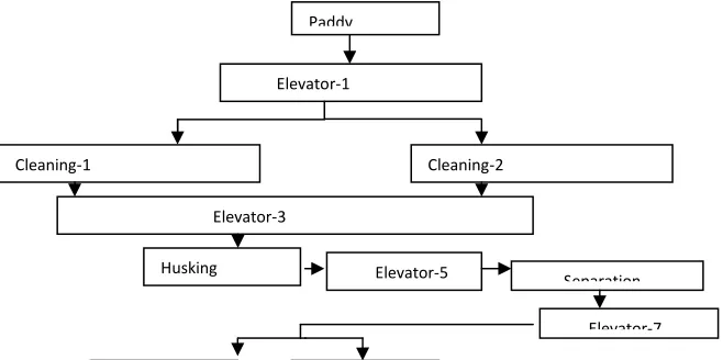
2.1 System description2.1.1 Sub-system E (Elevator)
Elevator (or lift) is vertical transport equipment that efficiently moves people or goods between floors These are five units ( , = 1,3,5,7,9).Failure of any one unit causes complete failure of the system.
2.1.2 Sub-system C (Cleaning)
.These are two identical units ( , = 1,2 )working in parallel.This unit can work with one unit in reduced capacity.
2.1.3 Sub-system H (Husking)
There is one unit subjected to major failure.
2.1.4 Sub-system S (Separation)
There is one unit subjected to major failure.
2.1.5 Sub-system W (Whitening)
These are two identical units ( , = 1,2) working in parallel. This unit can work with one unit in reduced capacity.
2.1.6 Sub-system L (Polishing)
These are two units ( , = 10,11).Failure of any one unit causes complete failure of the system.
2.2 Notations
−∶ The Sub-system/unit is running without any failure.
g: Unit is in good state but not operative. m: Unit is under preventive maintenance. r: unit is under repair or repair continued.
: ( = , ) indicate the working state of
husking separation machine w.r.t z,(z=-,g, m ,r).
: indicates the working state of the sub-system and w.r.t , , ( , = −, , ) ∶ : =
12 : indicates the working states of the subsystem L the ordered pair ( ) .1 and ( ) /0.1 represents the functioning of the sub-system L w. r. t to “t” and “n”(3 = 1,2; 4, = −, ).
5 /0512 : indicates the working states of the subsystem W the ordered pair ( ) 51 and ( ) /051
represents the functioning of the sub-system W w. r. t to “t” and “n”(6 = 1,2; 4, = −, ). 7 ( ): refers failure rate of the sub-system
8, /, 9, :, ;, 8<, 88, , and from normal to failed state ( = 1,3,5,7,9,10,11,12,13). 7(( ): refers failure rate of the sub-system and from normal to reduced state (* = 2,4).
7): refers constant transition state of the
subsystem and which transits the system into the 6 and 7 respectively on reaching to these state
preventing maintenance of H and S states start immediately, (, = 6,8).
µ ( ): Time dependent repair rates of the
subsystem 8, >, /, 9, :, ;, '8<, '88, , and to return it from failed to normal state and elapsed repair time is x,( = 1,3,5,7,9,10,11,12,13)
µ(( ): Time dependent repair rates of the subsystem and to return it from reduced to normal state and elapsed repair time “x”(* = 2,4).
?: Probability the PM of H and S is carried out satisfactorily and this makes the system operative( = 6,8).
1 − ?: Probability the PM of H and S is carried out unsatisfactory and this makes the system to failed state thereafter ( = 6,8).
The assumptions, on which the present analysis is based on, are as follows:
71
(ii) Failure and Repair rates of the subsystems are taken as variable.
(iii) Performance wise, a repaired unit is as good as new one for a specified duration..
(iv) Sufficient repair facilities are provided. (v) Service of the subsystem includes repair and/or replacement.
(vi) System may work at reduced capacity also.
3 Mathematical modeling of the system in transient state
Mathematical modeling has been developed for the prediction of time dependent availability of the individual components as well as entire system. The failure and repair rates of different subsystem available from the maintenance sheets of rice plant, are used us standard input information for Kumar et al (1999)The state of the system defines the condition at any instant of time and the information is useful in analyzing the current state and in the prediction of the failure state of the system. If the state of the is
3.1 When both failure and repair rates are variable
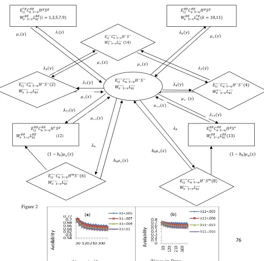
In this section we develop the Chapman-Kolmogorov differential equation assuming variable failure and repair rates of the subsystems by applying supplementary variable technique. In the transient state, Probability considerations give the following system of differential difference equation associated with the state transition diagram (fig. 1) of the system at time (4 + ∆4). Using mnemonic rule, we have 1,2,3,4,5,7,9,10,11,12,13
72
' ( , 0) = 0 ; = 6,8 ; ' ( , , 0) = 0 ; =
1,2,3,4,5,7,9,10,11,12,13,14 (14)
Solving these equations (1-9) together with initial and boundary conditions (10-14) using Lagrange’s method, we get the state probabilities as given below: '<(4) = T0UM1[1 + C <(4)TUM1E4]
If the industry provide the failure and repair rates, one can calculate the availability e5(4) in term of the probability'<(4), which is shown in equitation (1), thus, the time dependent availability e5(4) of the system is given by
e5(4)='<(4) + C ∑>,S,8SG> ' ( , , 4)E E +
C ∑GH,I' ( , 4)E (26)
73
Most of the authors have used Laplace transformation for simple systems and matrix method to solve the reliability function. But in this case it is difficult to find Laplace inverses, since expressions for probability transforms are in very complicated form and the complexity increase with the increase in number of equation. To overcome such type of problems the system of differential equation (27-33) with initial conditions (34) has been solved numerically following the approach adopted by Gupta et. al. (2007).Vaderperre and Makhanov(2005) used a numerical method to find the long run availability of a priority system.The numerical computation has been carried out starting from 4 = 0 to4 = 360 days assuming 4 = 0.005as equivalent to one day. The availability of rice mill has been obtained by taking different combinations of the constant failure and repair rates of the subsystems
3.3 Steady state availability when failure and repair rates are constant under idealized preventive maintenance
In the process industry, management remains interested in long run availability of the system.. This can be achieved by taking P1P → 0 andR1R → 0, as4 → ∞. Then the equations (1-9) reduce to linear algebraic equations when transitions rates are constant.
[∑ 78/ Solving recursively the above system of equations (36-40), we get Now using normalizing condition
74
and, the availability is ,
e5= f1 + p8+ p>+ p/+qµrr+
4 Performance Analyses
4.1 When Rates are Constant
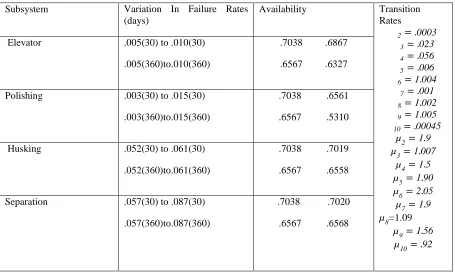
Figure 3(a) shows the availability of the system with failure rate78 of the Elevator for a period 360days divided over an interval of 30days. It seems that increase in failure rate (78) of elevator from .005 (once in 200 hrs.) to .010 (once in 100 hrs.) affect the availability of the system by (2.4% 4_ 3.6%) whereas it affect (6.6% 4_ 7.8%)with the increase in time from (30 Ea k4_ 360 Ea k)respectively
Figure 3(?) showsthat the availability decreases (6.7% to 19.1%) with the increase in the values of failure rate (788)of polishing machine from .003 (once in 333 days) to .014 (once in 7hrs.)respectively. Further we also find that when the time increase from (30 Ea k4_ 360 Ea k )the availability decrease by (6.7% t0 19.0%) respectively.
Figure 3(d) shows that availability of the system is affected by . 26% 40 .15% with the increase in failure rate (78>) of husking machine (once in 19hrs. to once in 16 hrs.) whereas increase in time affect it by app.
(6.6% 4_ 6.4%)from 30 days to 360 days respectively
Figure 3(E) shows that the availability decreases(.25% 4_ .13%) with the increase in the failure rate of separating machine (78/) from(.057 4_ .087)respectively . Further we also find that when the time increase from 30 days to 360 days the availability decrease by (6.6% 4_ 6.5%) respectively.
Figure 4(a) shows that the affect of repair rate of elevator on availability of the system. One can see that increase in time from 30 days to 360 days decrease the availability of the system decreases (8.4% 4_ 4.4%) however increase in repair rate (µ8) of elevator from .029(Once in 35hrs.)to. 04(once in 25hrs.) increase it app. (.68% 4_ 2.1%)
Figure 4(b) shows that the increase in repair rate (µ88) of polishing machine from .011 (once in 90 hrs.) to .10(once in 10hrs.) increase the availability of the system by (1.8% to 7.4%) and when the time increase from 30 days to 360days the availability decrease (8.4% to 3.3%).
Figure 4(c) shows that increase (1.1% t0 .97%) respectively with the increase in repair rate (µ8>) of husking machine from (1.10 4_ 4.10) .Further we also find that when the time increase from 30 days to 360 days the availability of the system decrease by app. (8.4% 4_ 8.5% respectively.
Figure 4(d) shows that the availability increases(.39% 4_ .35% ) with the increase in repair rate (µ8/) of separating machine from2.5 4_ 3.5. respectively Further we also find that by an increase in time from 30 days to 360 days the availability of the system decrease by app. 8.4% respectively.
4.2 Steady State Behavior
Figure 5(a) shows that behavior of availability of the system. Failure rate of elevator from different values of repair rate (µ8) of theelevator. It is included that increase in failure rate(78) from (.005 to .010) reduce the system availability by (3.6%) and the when repair rate (b1) of elevator is increasedfrom .029 to .119 the availability increase by (2.9%).
Figure 5(b) shows that the availability decrease in the by (23.1% and 9.5%) with the increase in the failure rate 788 of polishing machine from (.003 to .018)respectively. Further we also see that when repair rate (µ88) of polishing machine is increased from (.011 to .10) the availability of the system increase by (5.7% to 50.5%) respectively.
Figure 5(c) shows that the increase in failure rate (78>). Husking machine from (.57% to 0.16%) decrease availability of the system (.39%) and when repair rate µ8> of slicing machine increase from (1.10 to 4.10) the availability increase by .78%.
Figure 5(d) shows that the availability decreases by system increase by (.29% 4_ .71%) respectively.
5 Conclusions
75
difficulties in modeling and evaluating the performance of the system, especially during strategic maintenance planning. Through rigorous efforts have been made by researchers to evolve methods to study the effect of subsystem conditions and maintenance policies on system performance, these methods involve complex computations and the computations grow tremendously with further growth in number of subsystems.
Thus the above study shows that the availability tables and graphs provides us information about the system to be cared more and sequence of subsystem in which we should care. Thus the system will work
satisfactory for long time giving maximum output and also will improve the quality.
The performance analysis of rice mill help in increasing the production and quality of rice. Detailed study reveals that the polishing subsystem is critical part of the system and needs utmost care of management. Thus, the concerned managers can plan and adapt suitable maintenance practices/strategies for improving the system performance. Apart from these advantages the system performance analysis may help to conduct cost benefit analysis, operational capability studies, inventory spare parts management and replacement decisions.
References
1. Barlow, R.E. and Hunter ,L.C. Optimum preventive maintenance policies ;Operational Research 1960:8: 236-238.
2. Singh, Jai . Reliability consideration of Agro- industrial system using a heuristic approach ;CSIR New Delhi Project:1983. 3. Khan,N.M. and Gupta,A: Availability
analysis of 3 state system: IEEE Transactions on Reliability!985: R-34(1).
4. Michelsen, Q. Use of reliability technology in the process industry: Reliability Engineering and System Safety: 1998:60:179-181.
5. Zhao,M. Availability for repairable components and series system. IEEE Transictions on Relability 1994:2:43. 6. Priel, V.Z. Twenty ways to track
maintenance performance, Facotry :McGraw-Hill: 1974:81-91.
7. Osaki, S. and Nakagava, T. Bibliography for reliability and availability of stochastic system: IEEE Transaction On reliability :1976:25(4):284-287.
8. Hibi,S: How to measure maintenance performance: Asian Productivity Organization:1977.
9. Gupta P, Lal AK, Sharma RK, Singh J. Analysis of reliability and availability of serial processes of plastic-pipe manufacturing plant-a case study. International Journal of Quality and Reliability Management. 2007;24(4):404-419.
10. Singh,J.Reliability Technology-Theory and Applications(2ndEdition)I.K.International ,New Delhi India),2011.
11. Kumar,S.,Kumar,D. and Mehta,N.P. Maintenance management for ammonia synthesis system in a urea fertilizer plant.International Journal of Management and System 1999;15,211-214.
12. Ramakrishna,A. and Bawa,A.S. Optimization of machine design criteria for higher reliability and maintainability in food processing. Proc. International Conference on Reliability and Safety Engineering;2005;151-157.
13. Vanderperre,J.E. and Makhanov,S.S.. Long Run availability of priority system. A numerical approach,(2005);MPE1;355-364.
Figure Captions
Figure 1 Flow diagram of Rice plant. Figure 2 Transition diagram of rice plant
Figure 3 Effect of failure rates on availability of rice plant. Figure 4Effect of repair rates on availability of rice plant.
Figure 5 Effect of failure and repair rates on steady state availability of rice plant.
76
Figure 1
Figure 2
00
. /0.00 0 •(8) 5 /0500 ()00
00
. /0.00 • 0(6) 5 /0500 ()00
00
. /0.00 0 0(4) 5 /05‚0 00()
ƒƒ
. /0.ƒƒ ƒ ‚ 5 /05ƒƒ ()ƒƒ(13) ƒƒ
. /0.ƒƒ ‚ ƒ 5 /05ƒƒ ƒƒ() (12)
?HµH( )
?IµI( )
(1 − ?H)µH( ) (1 − ?I)µI( )
7H
78/( )
7I 00
. /0.‚0 0 0(2) 5 /0500 00()
µS ( ) µ>( )
µ8/( )
µ8>( )
78>( )
7>( ) 7S( )
00
. /0.‚0 0 0 5 /05‚0 00() (14)
µ( ) µ
(( )
µ>( ) µS( )
7S( ) 7>( )
7(( )
00
. /0.00 0 0 5 /0500 ()00
‚ƒ
. /0.ƒƒ ƒ ƒ
5 /05ƒƒ ()ƒƒ( = 1,3,5,7,9)
ƒƒ
. /0.ƒƒ ƒ ƒ 5 /05ƒƒ ‚ƒ()(* = 10,11)
77
Figure:3
79
0.029 0.059
0.089 0.119
0.005 0.009 0.61
0.62 0.63 0.64 0.65 0.66 0.67 0.68 0.69
Availability
Repair rate
Failure rate
(a) 0.68- 0.69
0.67- 0.68 0.66- 0.67 0.65- 0.66 0.64- 0.65 0.63- 0.64 0.62- 0.63 0.61- 0.62
0.01 0.04 0.07 0.1
0.003
0.013 0
0.1 0.2 0.3 0.4 0.5 0.6 0.7 0.8
Avalability
Repair rate F a ilure
R a te
(b) 0.7- 0.8
0.6- 0.7 0.5- 0.6 0.4- 0.5 0.3- 0.4 0.2- 0.3 0.1-0.2 0- 0.1
80
Figur:5
Figure5
Name of subsystem Failure rate (per hour) Repair rate(per hour)
Elevator1 78= .005 − .010 µ8= .029 − 0.04
Cleaning Machine 7>= .0003 − .0009 µ>= 1.5 − 1.9
Elevator-3 7/= .023 − .076 µ/= 1.001 − 1.007
Whitening Machine 7S= .056 − .086 µS= .90 − 1.5
Elevator-5 79= .002 − .006 µ9= .90 − 1.9
Husking Machine to normal to
maintenance 7H= 1.004 − 1.008
µH= 1.08 − 2.05
Elevator-7 7:= .001 − .008 µ:= 1.3 − 1.9
Separation Machine normal To maintenance
7I=1.002-1.006 µI=1.03-1.09
Elevator -9 7;= 1.005 − 1.009 µ;= 1.03 − 1.56
Polishing -10 78<= .00045-.00085 µ8<= .51 − .92
Polishing -11 788= .003 − .016 µ88= .011 − .10
Husking Machine to normal to failed
12= .052− .061 µ12 =1.10−4.10
Separation Machine normal to failed
81
Table I Failure and Repair rates of the subsystems of rice plant.
Table-II Variation in the data of failure rates of some important subsystem .The value inside the bract’s denotes days
Subsystem Variation In Failure Rates (days)
Polishing .003(30) to .015(30) .003(360)to.015(360)
Separation .057(30) to .087(30) .057(360)to.087(360)
.7038 .7020 .6567 .6568
Subsystem Variation In Repair Rates (days) Transition Rates
Elevator .0 29(30) to .04(30) .029(360) to .04(360)
.6129 .6171 .5613 .5723
82
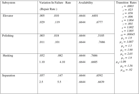
Table IIIVariation in the data of failure rates of the subsystem .The value inside the bract’s denotes days Subsystem Variation In Failure Rate
.(Repair Rate )
Availability Transition Rates
2 = .0003 3= .023 4= .056 5= .006 6 =1.004
7= .001 8 =1.002 9 =1.005 10= .00045
µ2=1.9 µ3=1.007
µ4=1.5 µ5=1.90 µ6=2.05 µ7=1.9 µ8=1.09
µ9=1.56 µ10= .92
Elevator .005 .010
.029 .119
.6644 .6401
.6644 .6777
Polishing .003 .018
.011 .101
.6644 .5105
.6644 .7686
Husking .052 .082
1.10 4.10 .6644 .7686
.6644 .6685
Separation .057 .147
2.5 5.5 .6644 .6592
.6644 .6639
Table IVVariation in the data of failure and repair rates of some important subsystem when both rates are constant. Separation 2.5(30) to 5.5(30) 2.5(360)to5.5(360) .6129 .6153