A Comparative Study of Two Procedures for Calculating Likelihood
Ratio in Forensic Text Comparison:
Multivariate Kernel Density vs.
Gaussian Mixture Model-Universal Background Model
Shunichi Ishihara Department of Linguistics Australian National University [email protected]
Abstract
We compared the performances of two proce-dures for calculating the likelihood ratio (LR) on the same set of text data. The first proce-dure was a multivariate kernel density (MVKD) procedure which has been success-fully applied to various types of forensic evi-dence, including glass fragments, handwriting, fingerprint, voice, and texts. The second pro-cedure was a Gaussian mixture model – uni-versal background model (GMM-UBM), which has been commonly used in forensic voice comparison (FVC) with so-called auto-matic features. Previous studies have applied the MVKD system to electronically-generated texts to estimate LRs, but so far no previous studies seem to have applied the GMM-UBM system to such texts. It has been reported that the latter GMM-UBM system outperforms the MVKD system in FVC. The data used for this study was chatlog messages collected from 115 authors, which were divided into test, background and development databases. Three different sample sizes of 500, 1500 and 2500 words were used to investigate how the per-formance is susceptible to the sample size. Re-sults show that regardless of sample size, the performance of the GMM-UBM system was better than that of the MVKD system with re-spect to both validity (= accuracy) (of which the metric is the log-likelihood-ratio cost, Cllr)
and reliability (= precision) (of which the met-ric is the 95% credible interval, CI).
1 Introduction
There are a large number of authorship analysis studies claiming to be forensic, particularly in the fields of computational linguistics and natural language processing (Iqbal et al. 2008, Iqbal et al. 2010, Lambers & Veenman 2009, Teng et al. 2004). Although they describe highly
sophisti-cated statistical and computational methodolo-gies, many of them consider the problem as a classification problem: for example, whether a system correctly identifies text as having been written by the same author or by different au-thors, etc. However, it is critical to appreciate that the role of the forensic scientist in this situa-tion is not to give a definitive answer to the ques-tion of authorship or to give an opinion on the likely authorship (whether the incriminating text was written by the suspect or not). This is the task of the trier-of-fact. (Aitken 1995, Aitken & Stoney 1991, Aitken & Taroni 2004, Robertson & Vignaux 1995). The above point is empha-sised in the following quote.
It is very tempting when assessing evidence to try to determine a value for the probabil-ity of guilt of a suspect, or the value for the odds in favour of guilt and perhaps even reach a decision regarding the suspect’s guilt. However, this is the role of the jury and/or judge. It is not the role of forensic scientist or statistical expert witness to give an opinion on this (Aitken 1995: 4).
So, what is the role of the forensic scientist? Aitken and Stoney (1991), Aitken and Taroni (2004) and Robertson and Vignaux (1995) state that the role of forensic scientist is to estimate the strength of evidence, technically called the likelihood ratio (LR).
This paper employs the LR framework, which has been advocated in major textbooks (e.g. Robertson & Vignaux 1995) and by forensic stat-isticians (e.g. Aitken & Stoney 1991, Aitken & Taroni 2004) as a logically and legally correct way of analysing and presenting forensic evi-dence. The LR framework is also the standard framework in DNA profiling. Emulating DNA forensic science, many fields of forensic
es, such as fingerprint (Neumann et al. 2007), handwriting (Bozza et al. 2008), voice (Morrison 2009) and so on, have started adopting the LR framework to quantify evidential strength (= LR).
Researchers engaged in forensic authorship analysis are well aware of LR and its importance in forensic comparative science. For example, the word ‘LR’ appears many times in papers, included in the 2nd issue of volume 21 of Journal of Law and Policy, which was published in 2013 as the proceedings of the papers presented at a forensic authorship attribution workshop1 held in October 2012. However, LR-based studies on forensic authorship analysis are conspicuous in their rarity. To the best of our knowledge, only a handful of studies so far have been based on the LR framework (e.g. Ishihara 2011, 2012a, b, Grant 2007).
There are several different procedures for cal-culating LRs (e.g. Lindley 1977, Aitken & Lucy 2004, Reynolds et al. 2000, Ishihara & Kinoshita 2010, Ishihara 2011). The Multivariate Kernel Density (MVKD) procedure is a popular one which has been successfully applied to various types of forensic evidence, such as voice (Rose et al. 2004), handwriting (Bozza et al. 2008) and text messages (Ishihara 2012b). Approaches based on Gaussian Mixture Model (GMM) are commonly used in forensic voice comparison (FVC) (Meuwly & Drygajlo 2001) and, in par-ticular, it was reported that the adapted version of the GMM procedure, namely the Gaussian Mixture Model - University Background Model (GMM-UBM) procedure outperformed the MVKD procedure in FVC (Morrison 2011a). However, to the best of our knowledge, the GMM-UBM procedure has not been applied to texts yet.
Thus, the first aim of this study is to test the GMM-UBM procedure for use on electronically-generated texts, more specifically chatlog mes-sages, in order to investigate how the GMM-UBM procedure performs in comparison to the MVKD procedure. The second aim is to investi-gate how their performance is influenced by sample size.
The performance of these procedures was as-sessed in terms of the log-likelihood-ratio cost (Cllr) (Brümmer & du Preez 2006) and the 95%
credible interval (CI) (Morrison 2011b) (see §3.5).
1
http://www.brooklaw.edu/newsandevents/events/2012/10-11-2012a.aspx
We have called our study ‘Forensic Text Comparison (FTC)’ study, instead of using the term ‘forensic authorship analysis’, to emphasise that the task of the forensic expert is to estimate and present the strength of evidence (= LR) in order to assist the decision of the trier-of-fact.
2 Likelihood Ratio
The LR is the probability that the evidence would occur if an assertion was true, relative to the probability that the same evidence would oc-cur if the assertion was not true (Robertson & Vignaux 1995).Thus, the LR can be expressed as 1).
For FTC, it will be the probability of observ-ing the difference (referred to as the evidence, E) between the offender’s and the suspect’s samples if they had come from the same author (Hp) (i.e.
if the prosecution hypothesis is true) relative to the probability of observing the same evidence (E) if they had been produced by different au-thors (Hd) (i.e. if the defence hypothesis is true).
The relative strength of the given evidence with respect to the competing hypotheses (Hp vs. Hd)
is reflected in the magnitude of the LR. The more the LR deviates from unity (LR = 1; logLR = 0), the greater support for either the prosecution pothesis (LR > 1; logLR > 0) or the defence hy-pothesis (LR < 1; logLR < 0).
For example, an LR of 20 means that the evi-dence (= the difference between the offender and suspect samples) is 20 times more likely to occur if the offender and the suspect had been the same individual than if they had been different indi-viduals. Note that an LR value of 20 does not mean that the offender and the suspect are 20 times more likely to be the same person than dif-ferent people, given the evidence.
3 Testing
Two types of comparisons are necessary to as-sess the performance of an FTC system: one is so-called same-author comparisons (SA compar-isons) and the other is different-author compari-sons (DA comparicompari-sons). For SA comparicompari-sons, two groups of messages produced by the same author will be compared and evaluated with the derived LR. Given that they are written by the same author, it is expected that the derived LR is higher than 1. In DA comparisons, two groups of messages written by different authors will be
compared and evaluated. They are expected to receive LR lower than 1, given that they are writ-ten by different authors.
3.1 Database
In this study, we used an archive of chatlog mes-sages2 which is a collection of real pieces of chatlog evidence used to prosecute paedophiles. As of August 2013, the archive contains messag-es from 550 criminals (= authors). From the ar-chive, we used messages collected from 115 au-thors (Dall), which were reformatted for the
pre-sent study.
In order to set up SA and DA comparisons, we needed two non-contemporaneous groups of messages from each of the authors. For this, we added messages one by one from the chronologi-cally ordered messages to the groups. For one message group, we started from the top of the chronologically sorted messages, while for the other group of the same author, we started from the bottom, and then the two groups of messages were checked to see if they were truly non-contemporaneous.
The 115 authors of the Dall were divided into
three mutually-exclusive sub databases of the test database (Dtest = 39 authors), the background
da-tabase (Dbackground = 38 authors) and the
develop-ment database (Ddevelopment = 38 authors). The Dtest
is for assessing the performance of the FTC sys-tem; the Dbackground as the reference database for
calculating LRs, and the Ddevelopment is for
calibrat-ing the derived LRs for the SA and DA compari-sons of the Dtest. From the testing database (Dtest)
of 39 authors, we can conduct independent 39 SA and 1482 DA comparisons.
For the actual testing, we differentiate the number of words included in each message group; 500, 1500, and 2500, in order to investi-gate the second research aim. 500 means that each message group was modelled using a total of approximately 500 words. Since we cannot perfectly control the number of words appearing in one message, it needs to be approximately 500 words.
3.2 Text processing and feature extractions
The chatlog messages were tokenised using the WhitespaceTokenizer function of the Natural Language Toolkit3. As the name indicates, the WhitespaceTokenizer provides a simple tokenisa-tion based on whitespaces. Thus, messages were
2
http://pjfi.org/
3
http://nltk.org/
whitespace-tokenised one by one. A message may have contained two or more sentences, but the words of each message were treated as a se-quence of words without parsing them into sen-tences.
We used three different features in this study, of which the effectiveness has been proven in previous studies (Ishihara 2012a, b). They are:
the number of words appearing in each mes-sage;
the average character number per word in each message; and
the ratio of punctuation characters (, . ? ! ; : ’ ”) to the total number of characters in each message.
The results of Ishihara (2012a, b), in which the different permutations of 12 so-called word- and character-based lexical features were investigat-ed in their performances, showinvestigat-ed that 1) a vector of four to five features (not as many as 12) yield-ed the best performing results and 2) the above three features performed consistently well re-gardless of the sample size. Thus, the above-listed features were chosen.
3.3 Likelihood ratio procedures
As mentioned earlier, two different procedures were used in order to calculate LRs: the Multi-variate Kernel Density (MVKD) procedure (Aitken & Lucy 2004) and the Gaussian Mixture Model - Universal Background Model (GMM-UBM) procedure (Reynolds et al. 2000).
Multivariate kernel density (MVKD) proce-dure
Although the reader needs to refer to Aitken and Lucy (2004) for the full mathematical expo-sition of the formula, we would like to point out some important parts of the formula, having its application to this study in mind. The numerator of the MVLR formula (2) calculates the likeli-hood of evidence, which is the difference be-tween the offender and suspect samples (e.g. the difference between the message group produced by the offender and that by a suspect) when it is assumed that both of them came from the same origin (e.g. both message groups were produced by the same author, or the prosecution hypothesis (Hp) is true). For that, we need the mean vectors
of the offender and suspect samples which are denoted as ̅ ̅ respectively in the formula, and the within-group (= within-author) variance, which is given in the form of a vari-ance/covariance matrix (denoted as U in the for-mula). The same mean vectors of the offender and suspect samples ( ̅ ̅ ) and the between-group (= between-author) variance (denoted as C in the formula) are used in the denominator of the formula (3), to estimate the likelihood of get-ting the same evidence when it is assumed that
they are from different origins (e.g. the defence hypothesis (Hd) is true). These within-group and
between-group variances (U and C of the formu-la) are estimated from the Dbackground consisting of
38 authors (m = 38), from each message group from which the above-mentioned three feature values (a three-dimensional feature vector) (p = 3) were extracted.
The difference of two feature vectors is evalu-ated using a Mahalanobis distance of which the general form is the product ̅ ̅ ̅ ̅ in the formula (e.g. the difference between offender and suspect means ( ̅ ̅ ) = ̅ ̅ ̅ ̅ . The MVKD formu-la assumes normality for within-group variance while it uses a kernel density model for between-group variance. The remaining complexities of the formula result mainly from modelling a ker-nel density for the between-group variance.
Gaussian mixture model – universal back-ground mode (GMM-UBM)
A Gaussian mixture model (GMM) is a paramet-ric probability density function represented as a weighted sum of M component Gaussian densi-numerator of MVLR ( = true), p ̅ ̅ =
⁄ ⁄ ⁄ | | ̅ ̅ ̅ ̅
∑ ̅ {( ) } ̅
(2)
Denominator of MVLR ( = true), p ̅ ̅ =
∏ ⁄
∑ ̅ ̅ ̅ ̅
(3)
where m = number of groups (e.g. authors) in the background data;
p= number of assumed correlated variables measured on each object (e.g. message); ni= number of objects in each group in the background data;
xij= measurements constituting the background data =(xij1,…,xijp) T
, i = 1,…,m, j = 1,…,ni;
̅ = within-object means of the background data = ∑ ;
ylj = measurements constituting offender (l = 1) and suspect (l = 2) data = (ylj1,…,yljp) T
, l = 1,2, j = 1,…,nl;
̅ = offender (l = 1) and suspect (l = 2) means = ∑ , l = 1,2. U, C = within-group and between-group variance/covariance matrices;
Dl = offender (l = 1) and suspect (l = 2) variance/covariance matrices = , l = 1,2;
ties. In FTC, GMM parameters are estimated from the training data (e.g. suspect samples) us-ing the iterative Expectation-Maximisation (EM) algorithm with the maximum likelihood (ML) estimation. The main idea of the GMM-UBM is that the GMM, which was built in the above pro-cess for a suspect, is adapted to a universal back-ground model (UBM) which was built based on the Dbackground. This way of estimating GMM
pa-rameters is called Maximum A Posterior (MAP) estimation. The above process is mathematically represented in terms of GMM parameters: mix-ture weight ( ), mixture mean ( ) and mixture variance/covariance ( ) in (4), (5) and (6) respec-tively. The formulae given in (4), (5) and (6) are based on Reynolds et al. (2000), but modified for text data.
If a mixture component (i) of the UBM has a low count for the corresponding mixture compo-nent of a given author’s (n) sample, thus low in
, then . This will result in de-emphasising the parameters of this mixture com-ponent of the UBM, and emphasising the given author’s original GMM parameters.
A score, which was transformed to an LR us-ing a calibration technique (refer to §3.4) in a subsequent process, was calculated as the
rela-tive value of the adapted GMM function of the suspect and the UBM function at each of the val-ues extracted from the offender sample.
In this study, we conducted a series of experi-ments by altering the number of Gaussian com-ponents and the relevance factor (r) between 8 and 24. The number of iteration for the EM algo-rithm was set to 7.
3.4 Calibration
A logistic-regression calibration (Brümmer & du Preez 2006) was applied to the derived LRs (or scores) from the MVKD and GMM-UBM proce-dures. Given two sets of LRs (or scores) derived from the SS and DS comparisons and a decision boundary, calibration is a normalisation proce-dure involving linear monotonic shifting and scaling of the LRs relative to the decision bound-ary in order to minimise a cost function. The Fo-Cal toolkit4 was used for the logistic-regression calibration in this study (Brümmer & du Preez 2006). The logistic-regression weight was ob-tained from the Ddevelopment.
3.5 Evaluation of performance: validity and reliability
The performance of the FTC system was as-sessed using the log-likelihood-ratio cost (Cllr)
(Brümmer & du Preez 2006) and the 95% credi-ble intervals (CI) (Morrison 2011b) which are the metrics of validity and reliability respective-ly. Suppose that we have two authors and two sets of message groups for each of author. We denote the sets of messages as A1.1, A1.2, A2.1, and A2.2, where A = author, and 1 & 2 = the first set and the second set of messages (A1.1 refers to the first set of messages collected from (A)uthor1, and A1.2 the second set from that same author). From these sets, two independent DA comparisons are possible; A1.1 vs. A2.1 and A1.2 vs. A2.2. Suppose then that we conducted two separate FTC tests in the same way, but us-ing two different features (Features 1 and 2), and that we obtained the log10LRs given in Table 1 for these two DA comparisons.
4
https://sites.google.com/site/nikobrummer/focal
̂ [ ] (4)
̂ (5)
̂ (6)
where, , and = the weight, mean and variance/covariance of the i-th component of speaker n’s GMM;
, and = the weight, mean and variance/covariance of the i-th component of UBM;
̂ , ̂ and ̂ = the adapted weight, mean and variance/covariance of the i-th component of speaker n’s GMM;
= a data-dependent adaptation coefficient, which is defined as
;
r = a relevance factor which controls the mag-nitude of the adaptation step in each iteration; T = the number of background samples used to train UBM
is automatically computed over all adapted mixture weights to ensure that they sum to uni-ty.
DA comparison Feature 1 Feature 2
A1.1 vs. A2.1 -3.5 -2.1
A1.2 vs. A2.2 -3.3 0.2
Since the comparisons given in Table 1 are DA comparisons, the desired log10LR value is lower than 0, and the greater the negative log10LR value is, the better the system is since it more strongly supports the correct hypothesis. For Feature 1, both of the comparisons revealed log10LR < 0 while for Feature 2, only one of them showed a log10LR < 0. Feature 1 is better not only in that both log10LR values are smaller than 0 (supporting the correct hypothesis) but also in that their magnitude is a lot greater than the log10LR values of Feature 2. As a result it can be said that the validity (= accuracy) of Feature 1 is higher than that of Feature 2. This is the basic concept of validity.
As pointed out in §1, almost all previous stud-ies of forensic authorship analysis treated the problem as a two-way classification problem (correct vs. incorrect). Consequently the validity of the methodology has been assessed in terms of classification accuracy such as precision, recall, equal error rate (EER), F-score, etc. However, Morrison (2011b: 93) argues that these metrics based on classification-accuracy/classification-error rates are inappropriate for use within the LR framework because they implicitly refer to posterior probabilities, which is the province of the trier-of-fact, rather than LRs, which is the province of forensic scientists. Furthermore, “they are based on a categorical thresholding, error versus non-error, rather than a gradient strength of evidence.” Thus it has been argued that an appropriate metric for the validity of the LR-based forensic comparison system is the log-likelihood-ratio cost (Cllr), which is a gradient
metric based on LRs. See 7) for calculating Cllr
(Brümmer & du Preez 2006).
ll =
1 2
(
1
∑ l 2(1 1
i)
i =
1
∑ l 2(1 j)
j = )
7)
In 7), NHp and NHd are the numbers of SA and
of DA comparisons, and LRi and LRj are the LRs
derived from the SA and DA comparisons re-spectively. If the system is producing desired LRs, all the SA comparisons should produce LRs greater than 1, and the DA comparisons should produce LRs less than 1. In this approach, LRs which support counter-factual hypotheses are given a penalty. The size of this penalty is de-termined according to how significantly the LRs deviate from the neutral point. That is, an LR supporting a counter-factual hypothesis with
greater strength will be penalised more heavily than the ones whose strength is closer to the uni-ty, because it is more misleading. The FoCal toolkit4 was also used for calculating C
llr in this
study (Brümmer & du Preez 2006). The lower the Cllr value is, the better the performance.
Both of the DA comparisons given in Table 1 are the comparisons between A1 and A2. Thus one can expect that the LR values obtained for these two DA comparisons to be similar since they are comparing the same authors. However, one can see that the log10LR values based on Feature 1 are closer to each other (-3.5 and -3.3) than those log10LR values based on Feature 2. In other words, the reliability (= precision) of Fea-ture 1 is higher than that of FeaFea-ture 2. This is the basic concept of reliability.
As the metric of reliability (= precision), we used credible intervals which are the Bayesian analogue of frequentist confidence intervals. Fol-lowing Morrison (Morrison 2011b: 62), we cal-culated the 95% credible intervals (CI) using the parametric method on the DA comparison pairs.
That is, for each member of the pair of LRs from each DA pair of authors (xa and xb), the
mean value of the pair ( ̅) was subtracted, as shown in 8).
The equations given in 8) convert each abso-lute value (xa and xb) to a deviation-from-mean
value (ya and yb). Then, the deviation-from-mean
value from each DA comparison pair of authors was pooled altogether to calculate CI. The small-er the credible intsmall-ervals, the bettsmall-er the reliability.
Tippett plots were also used in this study to visually present the magnitude of the derived LRs, including both consistent-with-fact and contrary-to-fact LRs. A more detailed explana-tion of Tippett plots is given in §4, in which some Tippett plots are presented.
4 Experimental Results and Discussions
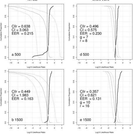
(r), displayed in Figure 1. Figure 1 also contains EER values, but these are only for reference.
We can observe from Figure 1 that regardless of the sample size, the GMM-UBM procedure outperforms the MVKD procedure in terms of both validity and reliability. However, the differ-ence in performance, in particular in validity, becomes less salient as the sample size increases. For example, the difference in Cllr between the
MVKD and GMM-UBM procedures is as large as 0.142 (= 0.638-0.496) when the sample size is
500, while the difference is only 0.026 (= 0.294-0.268) when the sample size is 2500. That is, when the sample size is small - which is more realistic in real casework - the GMM-UBM pro-cedure can be judged to be more appropriate to employ than the MVKD procedure.
Another clear difference between the two pro-cedures is that the MVKD produced greater LRs (with some extreme ones, e.g. LR > ) for the DA comparisons than the GMM-UBM, although the former is less well-calibrated than the latter.
MVLR GMM-UBM
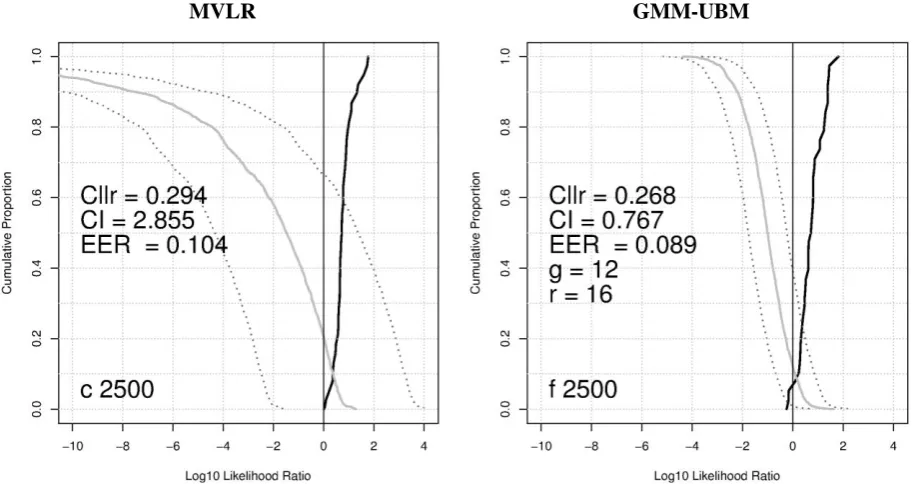
Figure 1: Tippett plots of the MVLR system on the left, and those of the GMM-UBM system (only best-performing ones) on the right. Sample size 500 (a,d); sample size 1500 (b,e). The calibrated SA LRs (solid black line), and the calibrated DA LRs (solid grey line) are plotted separately with the ±95% CI band (dotted grey lines) superimposed on the DA LRs. The Cllr, CI and EER values are also given in
[image:7.595.69.526.227.687.2]On the other hand, the LRs derived from the GMM-UBM are fairly conservative, in particular for the DA comparisons, but at the same time, their counter-factual LRs are also very weak. This point is particularly evident when the sam-ple size is small (500), in the sense that the DA LRs are overall greater in the MVKD than the GMM-UBM, whereas the former also produced greater contrarytofact SA LRs (e.g. LR = ca. -4). This led to heavy penalties in terms of validi-ty, resulting in a higher Cllr value (0.638) for the
MVKD system. The greater DA LRs for the MVKD procedure in comparison to the GMM-UBM procedure appears to be a general trend as the same trend has been reported in Morrison (2011a), in which these two procedures were compared on speech data.
As for the reliability of the system, the GMM-UBM is far better than the MVKD in that the CI is constantly less than 1 in the former whereas it can be higher than 3 in the latter. This higher CI value (= lower in reliability) of the MVKD sys-tem, being compared to the GMM-UBM, has also been pointed out in Morrison (2011a).
It is worth pointing out that although the GMM-UBM procedure performs better in validi-ty and reliabilivalidi-ty than the MVKD procedure, the LRs that the GMM-UBM estimated in the cur-rent study are fairly weak (this is also true of the MVKD procedure to a certain extent), in particu-lar from the view point that the log10LR between -1 and 1 can only provide limited support for either hypothesis. (Champod & Evett 2000). This is partly because only three features were used in
this study, but some previous studies (e.g. Ishihara 2012b) also reported that the LRs ob-tained from electronically-generated texts are relatively weak.
5 Conclusions and Future Directions
In this study, two procedures for the calculation of LRs: MVKD and GMM-UBM, were tested on the same feature set extracted from chatlog mes-sages, and their performance was compared in terms of validity (= accuracy) and reliability (= precision). The experimental results demonstrat-ed that the GMM-UBM system performdemonstrat-ed better in both validity and reliability than the MVKD system. Moreover, regardless of the sample size (500, 1500 and 2500 words), the reliability of the GMM-UBM system was consistently better than the MVKD system while the difference in validi-ty between the two procedures decreased as the sample size increased. Results also showed that although the GMM-UBM is generally better in performance than the MVKD, the magnitude of the DA LRs is more conservative in the former than the latter.
As mentioned in §1, there are several different procedures for estimating LRs. It would be worthwhile to test other procedures to see which procedure appears to be suited to text evidence.
Acknowledgments
The author greatly appreciates the very detailed comments of the three anonymous reviewers.
MVLR GMM-UBM
[image:8.595.69.527.74.316.2]References
Aitken CGG 1995 Statistics and the Evaluation of Evidence for Forensic Scientists John Wiley Chichester.
Aitken CGG & D Lucy 2004 'Evaluation of trace evidence in the form of multivariate data' Journal of the Royal Statistical Society Series C-Applied Statistics 53: 109-122.
Aitken CGG & DA Stoney 1991 The Use of Statistics in Forensic Science Ellis Horwood New York; London.
Aitken CGG & F Taroni 2004 Statistics and the Evaluation of Evidence for Forensic Scientists Wiley Chichester.
Bozza S, F Taroni, R Marquis & M Schmittbuhl 2008 'Probabilistic evaluation of handwriting evidence: Likelihood ratio for authorship' Journal of the Royal Statistical Society: Series C (Applied Statistics) 57(3): 329-341.
Brümmer N & J du Preez 2006 'Application-independent evaluation of speaker detection' Computer Speech and Language 20(2-3): 230-275.
Champod C & IW Evett 2000 'Commentary on A. P. A. Broeders (1999) ‘Some observations on the use of probability scales in forensic identification’, Forensic Linguistics 6(2): 228-41' International Journal of Speech Language and the Law 7(2): 238-243.
Grant T 2007 'Quantifying evidence in forensic authorship analysis' International Journal of Speech Language and the Law 14(1): 1-25.
Iqbal F, R Hadjidj, B Fung & M Debbabi 2008 'A novel approach of mining write-prints for authorship attribution in e-mail forensics' Digital Investigation 5(Supplement): S42-S51.
Iqbal F, LA Khan, BCM Fung & M Debbabi 2010 'E-mail authorship verification for forensic investigation' Proceedings of the 2010 ACM Symposium on Applied Computing: 1591-1598.
Ishihara S 2011 'A forensic authorship classification in SMS messages: A likelihood ratio based approach using N-gram' Proceedings of the Australasian Language Technology Workshop 2011: 47-56.
Ishihara S 2012a 'A forensic text comparison in SMS messages: A likelihood ratio approach with lexical features' Proceedings of the seventh International Workshop on Digital Forensics and Incident Analysis: 55-65.
Ishihara S 2012b 'Probabilistic evaluation of SMS messages as forensic evidence: Likelihood ration based approach with lexical features' International
Journal of Digital Crime and Forensics 4(3): 47-57.
Ishihara S & Y Kinoshita 2010 'Filler words as a speaker classification feature' Proceedings of the 13th Australasian International Conference on Speech Science and Technology: 34-37.
Lambers M & CJ Veenman 2009 'Forensic authorship attribution using compression distances to prototypes' in Z Geradts, KY Franke & CJ Veenman (eds) Computational Forensics Lecture Notes in Computer Science. Springer Link: 13-24.
Lindley DV 1977 'Problem in Forensic-Science' Biometrika 64(2): 207-213.
Meuwly D & A Drygajlo 2001 'Forensic speaker recognition based on a Bayesian framework and Gaussian Mixture Modelling (GMM)' Proceedings of 2001 Odyssey-The Speaker Recognition Workshop.
Morrison GS 2009 'Forensic voice comparison and the paradigm shift' Science & Justice 49(4): 298-308.
Morrison GS 2011a 'A comparison of procedures for the calculation of forensic likelihood ratios from acoustic-phonetic data Multivariate kernel density (MVKD) versus Gaussian mixture model-universal background model (GMM-UBM)' Speech Communication 53(2): 242-256.
Morrison GS 2011b 'Measuring the validity and reliability of forensic likelihood-ratio systems' Science & Justice 51(3): 91-98.
Neumann C, C Champod, R Puch-Solis, N Egli, A Anthonioz & A Bromage-Griffiths 2007 'Computation of likelihood ratios in fingerprint identification for configurations of any number of minutiae' Journal of forensic sciences 52(1): 54-64.
Reynolds DA, TF Quatieri & RB Dunn 2000 'Speaker verification using adapted Gaussian mixture models' Digital Signal Processing 10(1-3): 19-41.
Robertson B & GA Vignaux 1995 Interpreting Evidence: Evaluating Forensic Science in the Courtroom Wiley Chichester.
Rose P, D Lucy & T Osanai 2004 'Linguistic-acoustic forensic speaker identification with likelihood ratios from a multivariate hierarchical random effects model: A "non-idiot's Bayes" approach' Proceedings of the 10th Australian International Conference on Speech Science and Technology: 492-497.