Varro: An Algorithm and Toolkit for Regular Structure Discovery in
Treebanks
Scott Martens
Centrum voor Computerlingu¨ıstiek, KU Leuven [email protected]
Abstract
The Varro toolkit is a system for identi-fying and counting a major class of reg-ularity in treebanks and annotated nat-ural language data in the form of tree-structures: frequently recurring unordered subtrees. This software has been designed for use in linguistics to be maximally applicable to actually existing treebanks and other stores of tree-structurable nat-ural language data. It minimizes mem-ory use so that moderately large treebanks are tractable on commonly available com-puter hardware. This article introduces
condensed canonically ordered trees as a
data structure for efficiently discovering frequently recurring unordered subtrees.
1 Credits
This research is supported by the AMASS++ Project1 directly funded by the Institute for the
Promotion of Innovation by Science and Technol-ogy in Flanders (IWT) (SBO IWT 060051).
2 Introduction
Treebanks and similarly enhanced corpora are in-creasingly available for research, but these more complex structures are resistant to the techniques used in NLP for the statistical analysis of strings. This paper introduces a new treebank analysis suite Varro, named after Roman philologist Mar-cus Terentius Varro (116 BC-27 BC), who made linguistic regularity and irregularity central to his
1http://www.cs.kuleuven.be/˜liir/projects/amass/
philosophy of language in De Lingua Latina. (Harris and Taylor, 1989)
The Varro toolkit focuses on a general problem in performing statistical analyses on treebanks: identifying, counting and extracting the distribu-tions of frequently recurring unordered subtrees in treebanks. From this base, it is possible to con-struct more linguistically motivated schemes for performing treebank analysis. Complex statistical analyses are constructed from knowledge about frequency and distribution, so this constitutes a low level task on top of which higher level analy-ses can be performed.
An algorithm that can efficiently extract fre-quently recurring subtrees from treebanks has a number of immediate applications in computa-tional linguistics:
• Speeding up treebank search algorithms like Tgrep2. (Rohde, 2001)
• Rule discovery for tree transducers used in parsing and machine translation. (Knight and Graehl, 2005; Knight, 2007)
• Generalizing lexical statistics techniques in NLP – e.g., collocation – to a broader array of linguistic structures. (Sinclair, 1991)
• Efficiently identifying useful features for tree kernel methods. (Moschitti, 2006)
3 Theory and Previous Work
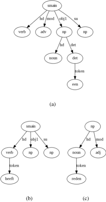
doubtless many other kind of linguistically moti-vated structures. Figure 1 is an example of a parse tree from a Dutch-language treebank.
Figure 1: A tree from the Europarl Dutch cor-pus. (Koehn, 2005) It has been parsed and labeled automatically by the Alpino parser. (van Noord, 2006) A word-for-word translation is “It also has
a legal reason.” (≈“There is also a legal reason
(for that).”)
In this paper, we are concerned with identify-ing and countidentify-ing frequent induced unordered
sub-trees in treebanks. The term subtree has a number
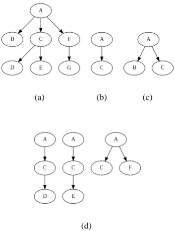
of definitions, but this paper will follow the ter-minology of Chi et al. (2004). Figure 2 contains three examples of induced unordered subtrees of the tree in Figure 1. Note that the ordering of the vertices in the subtrees is different from that of Figure 1. This is what makes them unordered
subtrees. Induced subtrees are more formally
de-scribed in Section 4.
3.1 Apriori
The research builds on frequent subtree discov-ery algorithms based on the well-known
Apri-ori algApri-orithm, which is used to discover
fre-quent itemsets in databases. (Agrawal et al., 1993) As a brief summary of Apriori, con-sider a collection of ordered itemsets C =
{{a, b, c},{a, b, d},{b, c, d, e}}. Apriori discov-ers all the subsets of those elements that appear at least some user-determinedθtimes. As an exam-ple, let us setθ = 2, and then count the number of times each unique item appears inC. Any sin-gle element inCthat appears less than two times cannot be a member of a set of elements that
ap-(a)
(b) (c)
Figure 2: Three induced unordered subtrees of the tree in Figure 1
pears at least θ times (since θ = 2), so those are rejected. Each of the remaining set elements
{a, b, c, d} is extended by counting the number of two-element sets that include it and some el-ement to the right in the ordered itemsets in C. For b, these are {{b, c},{b, d},{b, e}}. Of this set, only those that appear at leastθtimes are re-tained: {{b, c},{b, d}}. This process is repeated for size three sets, and iterated over and over for increasingly large subsets, until there are no ex-tensions that appear at leastθ times. This whole procedure is then repeated for each unique item. Finally, Apriori will have extracted and counted all itemsets that appear at leastθtimes inC.
(a) (b) (c)
(d)
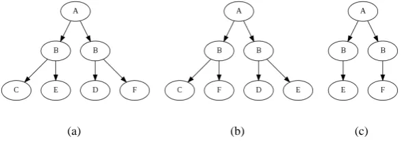
Figure 3: 3(b) and 3(c) are a subtrees of 3(a). The subtrees in 3(d) are possible extensions to 3(b), while 3(c) is not.
and counted by adding items to shorter and more frequent ones. This extends naturally to trees by initially locating and counting all the one-vertex trees in a treebank, and then constructing larger trees by adding vertices and edges to their right sides.
In Figure 3, subtree 3(b) has as valid extensions subtrees 3(d), all of which extend 3(b) to the right. An extension like subtree 3(c), which adds a node to the left of the rightmost node of 3(b), is not a valid extension.
3.2 Treebank applications
Applying these algorithms to natural language treebanks, however, presents a number of chal-lenges.
The approach described above, because it con-structs and tests subtrees by moving from left to right, is well-suited to finding ordered subtrees. However, this paper will consider unordered
sub-trees as better motivated linguistically. Word
or-der is not completely fixed in any language, and can be very free in many important contexts.
But there are other problems as well.
Apriori-style algorithms have the general property that their run-time is proportionate to the size of the output. Given a data-setDand a user-determined minimum frequency thresholdθ, this class of so-lution outputs all the patterns that appear at least θ times in D. If Dcontains n patterns that ap-pear at leastθtimes,P = {p1, p2, ..., pn};∀pi ∈
P : f req(pi) ≥ θ, then the time necessary to
identify and count all the patterns in P is pro-portionate to Pni=1f req(pi). In weakly
corre-lated data, this is a very efficient method of find-ing patterns. In highly correlated data, however, the number of patterns present can become pro-hibitively large and extend run-time to unaccept-able lengths, especially for smallθor large data-sets. Each frequent pattern may have any number of sub-patterns, each of which is also frequent and must be separately counted.
If we identify patterns with subtrees, a subtree with n vertices will, depending on its structure, have a minimum of n(n −1) and a maximum of(n−1)! + 1 subtrees. If each of those sub-trees is also a pattern that must be counted, then runtime grows very rapidly even for very small data-sets. Since natural language data is highly correlated, simple subtree-discovery extensions of
Apriori, like those proposed in (Zaki, 2002) and
(Asai, 2002), are not feasible for linguistic use. As reported in Martens (2009b), run-times become intractably long very quickly as data size increases for really existing treebanks.
However, there are compact representations of frequent patterns that are better suited to highly-correlated data and which can be efficiently dis-covered by modified Apriori schemes. This pa-per will only address one such representation:
fre-quent closures. (Boulicaut and Bykowski, 2000)
Frequent closures are widely used in subtree covery and have an intuitive meaning when dis-cussing natural language.
Given a treebankD, and a treeT that has a sup-port off req(T) = θ, thenT is closed if there is no supertreeT0 ⊃Twheref req(T0) =θ. In Fig-ure 3, if subtree 3(c) is as frequent in some tree-bank as 3(b), then 3(b) is not a closed subtree, nor can any further extension of it to the right be a closed subtree.
of English sentences, let us assume we have found a pattern of the form “NP make up NP to VP”, such as in “He has made up his mind to study
lin-guistics.” If every time this pattern appears in the
corpus, the second NP contains “mind”, then the pattern is not closed. A larger pattern appears just as often and in exactly the same places.
This makes the notion of frequent closed sub-tree discovery a generalization of collocation and
coligation - well known in corpus-based
lexicog-raphy - to arbitrary tree structures. (Sinclair, 1991) J.R. Firth famously said, “You shall know a word by the company it keeps.” (Firth, 1957) Frequent subtree discovery tells us exactly what company entire linguistic structures keep.
3.3 Efficient closed subtree discovery
Chi et al. (2005a) outlines a general method for ef-ficiently finding frequent closed subtrees without finding all frequent subtrees first. Their approach requires each subtree found to be aligned with its supertree before checking for closure and exten-sions. However, the alignment between a subtree and its supertree - the map from subtree vertices to supertree vertices - is not necessarily unique. A subtree may have a number of possible alignments with its supertree, even if one or more of the ver-tex alignments is specificed, as shown in Figure 4, which uses an example from the hand-corrected Alpino Treebank of Dutch.2
This can only be avoided by adding a restriction to trees: the combination of edge and vertex labels for each child of a vertex must be unique. This guarantees that specifying just one vertex in the alignment of a subtree to its supertree is enough to determine the entire unique mapping, but it is incompatible with most linguistic theories. Pro-cesses like tree binarization can meet this require-ment, but only with some loss of generality: Some frequent closed subtrees in a collection of trees like Figure 4(a) will no longer be frequent, or will be less frequent, in a collection of binary trees.
Martens (2009a) describes an alternative method of checking for closure which does not require alignment and can, consequently, be much faster. It has, however, two drawbacks: First, it does not find all frequent closed unordered
2http://www.let.rug.nl/vannoord/trees/
subtrees. Figure 5 shows the kind of tree where that approach is unable to correctly identify and count an unordered subtree. Second, it requires a great deal more memory than solutions that align each subtree discovered and check directly for closure, and is therefore of limited use with very large corpora.
4 Definitions
A fully-labeled rooted tree is a rooted tree in which each vertex and each edge has a label:T :=
hV, E, LV, LEi, whereV is the set of vertices,E
is the set of edges,LV is a mapLV : V → LV
from the vertices to a set of labels; and similarly LE maps the edges to labelsLE :E → LE. We
will designate an edgeeconnecting vertex v1 to
its childv2 by the notatione =hv1, v2i. LV and
LE constitute collectively the lexicon. Figure 1 is
an example of a fully-labelled, rooted tree from a Dutch-language treebank. This formalization is broadly applicable to all linguistic formalisms whose structures are tree-based or can be con-verted one-to-one into trees without loss of gener-ality. This may require some degree of restructur-ing of the tree formats used in particular lrestructur-inguistic theories. For example, in many formal linguistic theories, labels are not atomic symbols, but may have many parts or even whole structured feature sets. In general, these can be mapped to trees with atomic labels by inserting additional vertices, or by taking advantage of edge labelling.
The algorithm described here is insufficient for formal structures that require more powerful graph formalisms like directed acyclic graphs.
The relations parent, child and sibling are taken here in their ordinary sense in discussing trees. In Figure 1, the vertex labeled adv is a child of the vertex labeled smain, the parent of the vertex la-beled ook, and a sibling of the vertex lala-beled verb and the two vertices labeled np. To simplify defi-nitions, the operatorlabel(x)will indicate the la-bel of vertex or edgex.
An induced unordered subtree is a connected subset of the vertices of some tree that preserves the vertex and edge labels and the parent-child re-lations of that tree but need not preserve the or-dering of siblings. Given a fully-labeled treeT :=
(a) (b)
Figure 4: In 4(a) is a Dutch phrase conjoining multiple nouns. It translates as “police work, recreation,
planning and court activities”. 4(b) has six unique unordered alignments with 4(a).
(a) (b) (c)
Figure 5: Subtree 5(c) is an unordered subtree of both 5(a) and 5(b), but the algorithm described in Martens (2009a) is unable to capture this in all cases.
a fully-labeled treeS := hVS, ES, LVS, LESifor which there is an injection M : VS → VT from
the vertices ofSto some subset of the vertices of T, and for which:
∀v∈VS:
a. label(v) =label(M(v))
b. e=hparent(v), vi ∈ES →
e0 =hM(parent(v)), M(v)i ∈ET
c. label(e) =label(e0)
See Figures 1 and 2 for examples of subtrees of a particular tree.
We will further define all subtrees that are iden-tical except in the ordering of their vertices to be
unordered isomorphic. If a treeT is a subtree of tree T0, we will follow set notation by denoting this relation asT ⊆T0.
4.1 Canonical Ordering
Using canonical orderings to solve frequent un-ordered subtree problems was first proposed in Luccio et al. (2001) and expanded by other
researchers in frequent subtree discovery tech-niques, notably in Chi et al. (2005b). Since the
Apriori-style approaches described in Section 3.1
are suited only to finding subtrees whose vertices appear in a particular order, this paper will de-scribe a mechanism for converting fully-labeled trees into canonical forms that guarantee that all instances of any unordered subtree will have an identical order to their vertices.
We must first define a strict total ordering over vertex and edge labels. Given lexica for the edge and vertex labels, LE and LV respectively, we
define a strict total ordering on each such that
∀li, lj ∈ L either li ≺ lj or li lj or li = lj
and ifli ≺lj andlj ≺lk, thenli≺lk.
In a collection of fully-labeled trees, ev-ery vertex v that is not the root of some
tree can be associated with a full
la-bel which is the pair f ullLabel(v) =
order the vertices by the order of those edges. Where the edges are the same, we order them by the ordering of their vertex labels. Where we have two sibling vertices vi andvj such that
f ullLabel(vi) = f ullLabel(vj), we recursively
order the descendants of vi and vj, and then
compare them. In this way, two nodes can only have an undefined order if they have both exactly the same full labels and identical descendants.
A canonically ordered tree is a tree T :=
hVT, ET, LVT, LETi, where for eachv ∈ VT, the children ofvare ordered in just that fashion.
4.2 Condensed trees
A condensed tree is a fully-labeled tree T :=
hVT, ET, LVT, LETi with two additional proper-ties:
a. Each vertexv ∈ V is associated to a list of indices parentIndex(v) = {i1, i2, ..., in},
which we will call its parent index. Each en-tryi1, i2, ..., inis a non-negative integer.
b. No vertexv ∈ V has two children with the same full label.
Condensed trees are constructed from non-condensed trees as follows:
Given a tree T := hV, E, LV, LEi, we first
canonically order it, as described in the previous section. Then, we attach a parent index to each vertexv ∈V which is not the root ofT. The ini-tial parent index of each node consists of a single zero.
We then traverse the vertices of the now or-dered tree T in breadth-first order from the the root downwards and from left to right. Given some vj ∈ V, if it has no sibling to its right,
or if the sibling to its immediate right has a dif-ferent vertex label or a difdif-ferent edge label on the edge to its parent, we do nothing. Other-wise, if vj has a sibling to its immediate right
vi with the same full label, we set `i to the size
of parentIndex(vi), and then we append the
parentIndex(vj)toparentIndex(vi). Then, we
take the children ofvj, and for each one, we
incre-ment each value in its parent index by`i, and then
insert it undervias one ofvi’s children. We delete
vj and then we reorder the children ofvi into the
canonical order defined in Section 4.1.
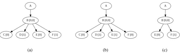
This is performed in breadth-first order overT. The result is guaranteed to be a tree where each vertex never has two children with the same edge and vertex labels. Figure 6 shows how the trees in Figure 5 look after they are converted into con-densed trees. We will denote concon-densed trees as T = cond(T), to indicate that T has been con-structed fromT.
If two non-condensed trees are unordered iso-morphic, then their condensed forms will be iden-tical, including in their vertex orderings and par-ent indexes. If two condensed trees are idpar-entical, then the non-condensed trees from which they are constructed are always unordered isomorphic.
Each vertexvof a condensed treeT=cond(T)
has a parent index containing some number of en-tries corresponding to a set of vertices in non-condensed tree T. We will designate that set as orig(v), a subset of the vertices inT. Given a condensed tree vertexvand its parentp, if the size oforig(p)is larger than one, then the vertices inv may have different parents inT. We can interpret the integers in the parent index of each condensed tree vertex as indicating which parent each mem-ber oforig(v)has.
In this way, given T = cond(T), there is a one-to-one mapping from the vertices of T to a pairhv, ii consisting of some vertex inT and an index to an entry in its parent index. If some vertex v in T maps to hv, ii, then all the chil-dren of v, c ∈ children(v) map to pairs hc, ji such that parent(c) = v and the jth entry in parentIndex(c) is i. We can use this to define parent-child operations over condensed trees that perfectly match parent-child operations in non-condensed ones.
We will define a skeleton tree as a con-densed tree stripped of its parent indices, and denote it as skel(T). Note that for any non-condensed tree T and any non-condensed sub-treeS ⊆ T, skel(cond(T))will always contain skel(cond(S)) as an ordered subtree, including in cases like Figure 5, as shown in Figure 6.
4.3 Alignment
(a) (b) (c)
Figure 6: The trees in Figure 5 transformed into their condensed equivalents, with their parent arrays. Note that 6(c) is visibly an ordered subtree of both 6(a) and 6(b) if you ignore the parent arrays.
a. Skeleton Alignment:
An injectionM :VS→VTfrom the vertices
ofSto the vertices ofT. b. Index Alignment:
For each vertex vS ∈ VS, a bipartite
map-ping from the vertices inorig(vS)to the
ver-tices inorig(M(vS)).
The first part is an alignment of skel(S)with skel(T). Given an alignment from the root ofS to some vertex inT, this can be performed in time proportionate, in the worst case, to the number of vertices inskel(T). If all the parent indices of the aligned vertices in the subtree and supertree have only one index in them, then the index alignment is trivial and the alignment ofStoTis complete. In other cases, index alignment is non-trival. The method here draws on the proce-dure for unordered subtree alignment proposed by Kilpel¨ainen (1992). In the worst case, it resolves to the same algorithm, but can perform better on the average because of the structure of condensed trees.
Alignment proceeds from the bottom-up, start-ing with the leaves ofS. If vertexs is a leaf of Sand is aligned to some vertex t inT, then we initially assume any member oforig(s) can map to any member oforig(t). We then proceed up-wards inS, checking each vertexsinSto find a mapping fromorig(s)toorig(t)such that if some s∈ orig(s)can be mapped to somet ∈orig(t), then the children ofscan be mapped to children oft.
Once we reach the root ofS, we proceed back downwards, removing those mappings from each orig(s)to its corresponding orig(t) that are im-possible because their parents do not align.
The remaining index alignments must still be checked to verify that each one can form a part of a one-to-one mapping fromorig(s)toorig(t). This is equivalent to finding a maximal bipar-tite matching from orig(s) to orig(t) for each possible alignment from orig(s) to orig(t). Bi-partite matching is a problem with a number of well-documented solutions. (Dijkstra (1959), Lov´asz (1986), among others)
5 Algorithm
Having outlined condensed trees and how to align them, we can build an algorithm for extracting all frequent closed unordered subtrees from a tree-bank of condensed trees, given a minimum fre-quency threshold θ. Space restrictions preclude a full formal description of the algorithm, but it closely follows the general outline for closed tree discovery schemes advanced by Chi et al. (2005a):
1. Pass through the treebank collecting all the subtrees that consist of a single vertex label and all their locations.
2. Remove those that appear less thanθtimes. 3. Loop over each remaining subtree, aligning
it to each place it appears in the treebank 4. Collect all the possible extensions, creating a
new list of two vertex subtrees and all their locations.
5. Use the extensions to the left of the rightmost vertex in each alignment to check if the sub-tree is closed to the left, and reject it if it is not.
7. Retain the extensions to the right of the right-most vertex and their locations if those exten-sions appear at leastθtimes.
8. Repeat for those subtrees.
6 Implementation and Performance
The Varro toolkit implements condensed trees and the algorithm described above in Python 3.1 and has been applied to treebanks as large as several hundred thousand sentences. The software and source code is available from sourceforge.net3and includes a small treebank of parsed Latin texts provided by the Perseus Digital Library. (Bam-man and Crane, 2007)
The worst case memory performance of this al-gorithm isO(nm)wherenis the number of ver-tices in the treebank andmis the largest frequent subtree found in it. However, only the most patho-logically structured treebank could come close to this ceiling, and in practice, the current implemen-tation has so far never used as much twice the memory required to store the original treebank.
The runtime performance is, as described in Section 3.2, proportionate to the size of the out-put. However, aligning each occurrence of each subtree adds an additional factor. Given a con-densed subtree S and its condensed supertree T containing size(T) vertices, and one already aligned vertex, the worst case alignment time is O(size(T)2.5), but only a highly pathological tree structure would approach this. The best case alignment time is O(size(S)). Therefore, it al-ways takes more time to align larger subtrees, and since larger subtrees are less frequent than smaller ones, setting lower minimum frequency thresh-olds increases the average time required to process a subtree.
Processing even the small Alpino Treebank produces very large numbers of frequent closed subtrees. After removing punctuation and the to-kens themselves, leaving just parts-of-speech and consituency labels - the Alpino treebank’s 7137 sentences are reduced to 206,520 vertices. Within this small set, Varro took 1252 seconds to find 7307 frequent closed subtrees that appear at least 100 times. This is both considerably more
sub-3http://varro.sourceforge.net/
trees than reported by Martens (2009b) on the same data and considerably more time.
Speed and memory performance are the major practical issues in this line of research. Choos-ing to design Varro with memory footprint mini-mization in mind is a source of some performance bottlenecks. Using Python also takes a heavy toll on speed and a C++ implementation is planned. The fast alignment-free closure checking scheme in Martens (2009b) can also be implemented us-ing condensed trees. On small treebanks this will improve speed without loss of precision, but has limited applicability to large treebanks.
7 Conclusions
The trade-off between memory usage, run-time and completeness for this kind of algorithm is
punitive. The user must balance very long
run-times against excessive memory usage if they want to accurately count all frequent unordered induced subtrees. The Varro toolkit is designed to make it possible to choose what tradeoffs to make. Since any subtree can be extended and checked for closure independently of other subtrees, Varro can easily implement heuristics designed to further re-duce the number of subtrees extracted. We believe the future of this line of research lies in large part in that direction and hope that public release of
Varro will aid in its development.
References
Agrawal, Rakesh, Tomasz Imielinski and Arun Swami. 1993. Mining association rules between sets of items in large databases. Proceedings of the 1993
ACM SIGMOD International Conference on Man-agement of Data, pp. 207–216.
Asai, Tatsuya, Kenji Abe, Shinji Kawasoe, Hiroki Arimura, Hiroshi Sakamoto and Setsuo Arikawa. 2002. Efficient substructure discovery from large semi-structured data. Proceedings of the Second SIAM International Conference on Data Mining,
158–174.
Bamman, David and Gregory Crane. 2007. The Latin Dependency Treebank in a Cultural Heritage Digital Library. Proceedings of the Workshop on Language Technology for Cul-tural Heritage Data, LaTeCH 2007: pp. 33–40.
http://nlp.perseus.tufts.edu/syntax/treebank/
Boulicaut, J.-F. and A. Bykowski. 2000. Frequent closures as a concise representation for binary data mining. Knowledge discovery and data mining: current issues and new applications, PAKDD 2000:
pp. 62–73.
Chi, Yun, Richard R. Muntz, Siegfried Nijssen and Joost N. Kok. 2004. Frequent Subtree Mining - An Overview. Fundamenta Informaticae, 66(1-2):161– 198.
Chi, Yun, Yi Xia, Yirong Yang and Richard R. Muntz. 2005a. Mining Closed and Maximal Frequent Subtrees from Databases of Labeled Rooted Trees.
IEEE Transactions on Knowledge and Data Engi-neering, 17(2):190–202.
Chi, Yun, Yi Xia, Yirong Yang and Richard R. Muntz. 2005b . Canonical forms for labelled trees and their applications in frequent subtree mining. Knowledge
and Information Systems, 8(2):203–234.
Dijkstra, E. W. 1959. A note on two problems in connexion with graphs. Numerische Mathematik
1:269–271.
Firth, J.R. 1957. Papers in Linguistics. London: OUP.
Harris, Roy and Talbot J. Taylor. 1989/1997. Varro on Linguistic Regularity. In Harris and Taylor,
Land-marks in Linguistic Thought I: The Western Tra-dition from Socrates to Saussure. 2nd ed. London:
Routledge. pp. 47-59.
Kilpel¨ainen, Pekka. 1992. Tree Matching Problems
with Applications to Structured Text Databases.
PhD dissertation. Univ. Helsinki, Dept. of Computer Science.
Knight, Kevin. 2007. Capturing practical natural language transformations. Machine Translation,
21:121–133.
Knight, Kevin and Graehl, Jonathan. 2005. An Overview of Probabilistic Tree Transducers for Nat-ural Language Processing. Proceedings of the 6th
CICLing, 1–24.
Koehn, Philipp. 2005. Europarl: A Parallel Corpus for Statistical Machine Translation. Proceedings of the
10th Machine Translation Summit, 79–86.
Lov´asz, L´aszl´o and M.D. Plummer. 1986. Matching
Theory. Amsterdam: Elsevier Science.
Luccio, Fabrizio, Antonio Enriquez, Pablo Rieumont and Linda Pagli. 2001. Exact Rooted Subtree Matching in Sublinear Time. Universit`a Di Pisa Technical Report TR-01-14.
Moschitti, Alessandro. Making tree kernels practical for natural language learning. Proceedings of the
11th Conference of the European Association for Computational Linguistics (EACL 2006), 113–120.
Mel’ˇcuk, Igor A. 1988. Dependency syntax: Theory
and practice. Albany, NY: SUNY Press.
Martens, Scott. 2009a. Frequent Structure Discovery in Treebanks. Proceedings of the 19th
Computa-tional Linguistics in the Netherlands (CLIN 19).
Martens, Scott 2009b. Quantitative analysis of treebanks using frequent subtree mining methods.
Proceedings of the 2009 Workshop on Graph-based Methods for Natural Language Processing (TextGraphs-4), 84–92.
Rohde, Douglas. 2001. Tgrep2 User Manual.
http://tedlab.mit.edu/∼dr/Tgrep2
Sinclair, John. 1991. Corpus, Concordance,
Colloca-tion. Oxford: OUP.
Tesni`ere, Lucien. 1959. El´ements de syntaxe struc-´ turale. Paris: ´Editions Klincksieck.
van Noord, Gertjan. 2006. At last parsing is now operational. Verbum Ex Machina. Actes de la 13e conf´erence sur le traitement automatique des langues naturelles (TALN6), 20–42.
Mohammed J. Zaki. 2002. Efficiently mining fre-quent trees in a forest. Proceedings of the 8th ACM