Abstract
McDANIEL, MATTHEW CARY. Characterizing Individual Response to Lipid Infusions using Time-Varying Physiological Parameters to Predict Lipid Resuscitation Outcomes. (Under the direction of Dr. Kevin Flores.)
Local anesthetic systemic toxicity (LAST) is a life-threatening event in which the
introduction of anesthetic to the bloodstream induces rapid onset of cardiac arrest. The
severity of this condition is compounded by its resistance to traditional methods of
re-suscitation. A potential remedy emerged twenty years ago when it was observed that
injecting rats with the solution Intralipid decreased their susceptibility to toxic events
caused by the anesthetic bupivacaine. The widespread clinical availability of Intralipid
made this phenomenon all the more intriguing. Momentum behind Intravenous Lipid
Emulsion (ILE) therapy built following further studies in animals and crescendoed in the
mid-2000s when it was implicated in the rescue of several patients from LAST.
Encouraging as some case studies have been, a contingent of the medical community
has expressed concern that positive reports have led to adoption of ILE therapy without
proper validation of its efficacy. They argue out that the biological mechanism by which
ILE therapy operates has not been fully elucidated and that the proposed “lipid sink”
theory cannot adequately explain all experimental observations. Furthermore, they point
to experiments in other animals that have produced conflicting results with respect to
the superiority of ILE therapy over traditional resuscitation techniques. This opposition
desires not to debunk ILE therapy, but to ensure that physicians understand when it
is appropriate to use it. This point is particularly critical when considering that ILE
therapy has already been attempted in oral rather than intravenous overdose cases, as
The purpose of our study was twofold. We first sought to demonstrate how
mathe-matical analysis can be used to gain insight into the mechanism by which ILE therapy
operates. In doing so, we establish how estimation of relevant physiological parameters on
an individual basis can inform personal treatment protocols and establish population level
trends. Using data previously collected in a study involving rats, we identified two key
pa-rameters in a compartmental, physiologically-based pharmacokinetic/pharmacodynamic
(PK/PD) model associated with lipid interactions that can be estimated for each
sub-ject. One parameter was determined to be correlated with the magnitude of cardiac
response to lipid infusion, while the other played a role in determining the smoothness
of the response. To account for the dynamic nature of the process, we adjusted the
PK/PD model to allow time variation in our selected parameters using one, four, or eight
linear splines of equal length. We evaluated the quality of our candidate models with
model comparison nested restraint tests and Akaike Information Criteria (AIC),
deter-mining that a model with four linear splines was most appropriate for our data set. We
constructed population distributions for each parameter using the individual estimates,
sampling from them repeatedly to create a virtual population undergoing ILE therapy in
response to a simulated overdose of the anesthetic bupivacaine. The virtual population
exhibited a wide range of expected outcome, demonstrating how the viability of ILE
therapy could depend strongly on the individual.
Future work will seek to expand the pool of parameters we are able to estimate to
increase the confidence which we can place on our virtual populations. Transitioning our
study to higher animal models is another logical step forward. We are confident that by
doing so we will contribute to the understanding of ILE therapy and provide a blueprint
Characterizing Individual Response to Lipid Infusions using Time-Varying Physiological Parameters to Predict Lipid Resuscitation Outcomes
by
Matthew Cary McDaniel
A thesis submitted to the Graduate Faculty of North Carolina State University
in partial fulfillment of the requirements for the Degree of
Master of Science
Biomathematics
Raleigh, North Carolina
2017
APPROVED BY:
Belinda Akpa Hien Tran
Kevin Flores
Biography
Matthew McDaniel was born in Phoenix, AZ. His parents loved him, so they moved to
Tucson rather than allow Matthew to suffer the ignominy of growing up an Arizona State
Acknowledgments
Thanks to Dr. Kevin Flores and Dr. Belinda Akpa for the opportunity to work on this
project and for all their support. Specifically, I’d like to acknowledge all the great input I
got from Kevin relating to the mathematical execution of our study and for being available
to talk at the drop of a hat. Dr. Akpa was instrumental in the process of transferring
the PK/PD model to a Matlab format that we could use to perform our study. She
also provided the data which we used for this study and was an excellent resource on
Table of Contents
List of Tables ... vi
List of Figures... vii
1 Review ... 1
1.1 Development of ILE Therapy . . . 1
1.2 Controversy Concerning ILE . . . 3
1.2.1 Mechanism . . . 3
1.2.2 Interactions with Vasopressors . . . 5
1.2.3 Scope and Safety . . . 7
1.2.4 The Need for a Better Model . . . 8
1.3 Mathematics in Clinical Settings . . . 9
1.3.1 PK/PD Models . . . 9
1.3.2 A PK/PD Model for ILE Therapy . . . 10
1.3.3 Personalized Medicine and Virtual Populations . . . 13
1.4 Goals of this Paper . . . 14
2 Parameter Estimation 1 ... 14
2.1 Data and Methods . . . 14
2.1.1 Data . . . 14
2.1.2 Cardiac Function Adjustment . . . 15
2.1.3 Inverse Problems . . . 16
2.1.4 Uncertainty Quantification and Subset Selection . . . 19
2.1.5 Time Varying Parameters . . . 20
2.2 Results . . . 23
2.3 Discussion . . . 38
3 Parameter Estimation 2 ... 41
3.1 Methods . . . 41
3.2 Results . . . 42
3.3 Discussion . . . 52
4 Virtual Population Studies ... 53
4.1 Methods . . . 53
4.2 Results . . . 54
4.3 Discussion . . . 56
5 Conclusions and Future Work... 57
List of Tables
Table 1: Candidate Parameters for Estimation in Individual Rat Response to
ILE Infusion . . . 15
Table 2: P-values for nested model comparison tests for each rat. In each test,
the first model listed is nested within the second, and a p-value of less
than 0.05 indicates that the second model is significantly improved over
the first. The model with four-spline representations of both n and α
is significantly superior to the constant model (Test 6), the one-spline
models (Tests 7-9), and the four-spline models with either n or α time
varying (Tests 10-11). Introduction of eight-spline representations of n
List of Figures
Figure 1: Physiologically Based Compartmental Pharmacokinetic Model for
Bupi-vacaine [29] . . . 11
Figure 2: Subset selection results for candidate parameters for estimation. Red
line denotes a normalized standard error less than 1
1.96. The colored circles indicate the combination of np parameters that produce the
low-est error. These results indicate that no more than two parameters can
be estimated with reasonable confidence from the available data. The
identities of these parameters are n and α. Results are with respect to
Subject 5 but are typical of all subjects . . . 24
Figure 3: Predicted cardiac output for rat 1 estimating n and α as (a) constant
parameters and as time varying parameters via (b), one, (c) four, and
(d) eight linear splines . . . 25
Figure 4: Predicted cardiac output for rat 2 estimating n and α as (a) constant
parameters and as time varying parameters via (b), one, (c) four, and
(d) eight linear splines . . . 26
Figure 5: Predicted cardiac output for rat 3 estimating n and α as (a) constant
parameters and as time varying parameters via (b), one, (c) four, and
(d) eight linear splines . . . 27
Figure 6: Predicted cardiac output for rat 4 estimating n and α as (a) constant
parameters and as time varying parameters via (b), one, (c) four, and
(d) eight linear splines . . . 28
Figure 7: Predicted cardiac output for rat 5 estimating n and α as (a) constant
parameters and as time varying parameters via (b), one, (c) four, and
Figure 8: Predicted cardiac output for rat 6 estimating n and α as (a) constant
parameters and as time varying parameters via (b), one, (c) four, and
(d) eight linear splines . . . 30
Figure 9: Predicted cardiac output for rat 7 estimating n and α as (a) constant
parameters and as time varying parameters via (b), one, (c) four, and
(d) eight linear splines . . . 31
Figure 10: Comparison of spline representations for the parameter n using (a) m
= 1 spline, (b) m = 4 splines, and (c) m = 8 splines . . . 32
Figure 11: Comparison of spline representations for the parameter α using (a) m
= 1, (b) m = 4 splines, and (c) m = 8 splines . . . 33
Figure 12: AIC Scores for Subjects 1-4 across models with time variation in
com-binations ofn and α for m = 1, 4, and 8 splines. Legend denotes which
variable is time varying . . . 34
Figure 13: AIC Scores for Subjects 5-7 across models with time variation in
com-binations ofn and α for m = 1, 4, and 8 splines. Legend denotes which
variable is time varying . . . 35
Figure 14: AIC Scores for all subjects using spline representations fornand α as a
function of the number of splines Used. The models using four and eight
splines produce very similarly appropriate fits for many of the subjects 36
Figure 15: Distributions of estimated node locations for four-spline representations
of (a)n and (b)αbased on N = 7 subjects. Red lines represent median
values; box boundaries define inner-quartile range (IQR); whiskers
de-fine min and max values within 1.5*IQR of median; red crosses denote
Figure 16: Predicted cardiac output for rat 1 estimating n and α as time varying
parameters with (a) two splines of unequal length parameters compared
to (b) one spline and (c) four splines of equal length . . . 43
Figure 17: Predicted cardiac output for rat 2 estimating n and α as time varying
parameters with (a) two splines of unequal length parameters compared
to (b) one spline and (c) four splines of equal length . . . 44
Figure 18: Predicted cardiac output for rat 3 estimating n and α as time varying
parameters with (a) two splines of unequal length parameters compared
to (b) one spline and (c) four splines of equal length . . . 45
Figure 19: Predicted cardiac output for rat 4 estimating n and α as time varying
parameters with (a) two splines of unequal length parameters compared
to (b) one spline and (c) four splines of equal length . . . 46
Figure 20: Predicted cardiac output for rat 5 estimating n and α as time varying
parameters with (a) two splines of unequal length parameters compared
to (b) one spline and (c) four splines of equal length . . . 47
Figure 21: Predicted cardiac output for rat 6 estimating n and α as time varying
parameters with (a) two splines of unequal length parameters compared
to (b) one spline and (c) four splines of equal length . . . 48
Figure 22: Predicted cardiac output for rat 7 estimating n and α as time varying
parameters with (a) two splines of unequal length parameters compared
to (b) one spline and (c) four splines of equal length . . . 49
Figure 23: AIC Scores for Subjects 1-4 across models with time variation in
com-binations of n and α for m = 1, 4, and 8 splines. Updated to include
Figure 24: AIC Scores for Subjects 5-7 across models with time variation in
com-binations of n and α for m = 1, 4, and 8 splines. Updated to include
model with 2 splines of unequal length (2∗) . . . 51
Figure 25: Virtual population of rats treated with 20% Intralipid in response to
bupivacaine infusion using model with four-spline representations of n
and α. Bupivacaine overdose modeled as 10 mg/kg administered at
constant rate from time t = 0 to t = 20 seconds. Lipid treatment
modeled as 4 mg/kg administered at constant rate from time t =30
to t = 50 seconds. Solid line = median, dotted lines = middle 50th
percentile, dashed lines = middle 95th percentile . . . 54
Figure 26: Virtual population of rats treated with 30% Intralipid in response to
bupivacaine infusion. Bupivacaine overdose modeled as 10 mg/kg
ad-ministered at constant rate from time t = 0 to t = 20 seconds. Lipid
treatment modeled as 4 mg/kg administered at constant rate from time
t =30 to t = 50 seconds. Black line = median, blue dotted lines =
1
Review
1.1
Development of ILE Therapy
The use of local anesthesia is an established operating procedure in clinical settings.
Local anesthetics–which come in the form of topical applications, local infiltration, and
nerve blocks[28]-very rarely produce adverse side effects. Yet when they do, the risk to a
patient’s life is extreme. If a local anesthetic enters bloodstream, usually by inadvertent
infusion, central nervous system and cardiac toxicity can result [41]. The severity of
local anesthetic system toxicity (LAST), as it is called, stems from its strong negative
inotropic effect on the heart [6]. That is, LAST weakens the cardiac muscle tissue.
To further complicate matters, individuals experiencing LAST do not respond well to
traditional resuscitation methods [46]. Concern over this issue was first brought to light
by Stephen Albright of Stanford Medical Center in 1979. Albright expressed doubts that
standard resuscitation protocol could mitigate cardiac arrest induced by ”potent, highly
lipid soluble and protein-bound amide...agents such as etidocaine and bupivacaine” [1].
Yet in the absence of a realistic alternative, the agents referenced by Albright remain
widely used. As of 2013, estimated incidence of LAST was 0.87 out of 1000 patients [5].
Interestingly, the lipophillic property cited by Albright as playing a role in LAST
might hold the key to combating it. Weinberg et al observed in 1998 that the mean
lethal dosage of bupivacaine required to induce asystole [i.e. flat-line] in rats could be
increased by pre-treating the animals with an intravenously injected lipid emulsion [53].
The solution in question was Intralipid, which is commonly used as a source of free
fatty acids in parenteral nutrition [49]. Weinberg postulated that the Intralipid acts as
[53]. In vitro experiments appeared to support this lipid sink theory, as the lipid:aqueous
partition coefficient for bupivacaine was found to be 11.9. In a follow-up study performed
with dogs, all animals treated with Intralipid survived bupivacaine-induced cardiotoxity
compared to none in the control group [52]. At this juncture, an editorial raised the
question of whether Intravenous Lipid Emulsion (ILE) therapy might represent the ”silver
bullet” in treating LAST [50].
Enthusiasm heightened in 2006 when ILE therapy was successfully applied for the
first time in a clinical setting [45]. A male patient went into cardiac arrest after receiving
bupivacaine and, after 20 minutes of standard resuscitation protocol, could not be revived.
The patient was given a 100 mL bolus infusion of 20% Intralipid and, within seconds,
began showing signs of recovery. Further stabilization of the patient was achieved by
administering a continuous infusion of lipid. Over the next several years, subsequent
case studies were published describing reversal of cardiac toxicity brought about by a
range of anesthetics, including levobupivacaine [18], mepivacaine [34], prilocaine [34],
ropivacaine [35], and lidocaine [35]. In each case, reversal was accomplished using a
regimen of a bolus infusion of lipid followed by a continuous infusion.
Each documented rescue event has been received by many as more evidence in favor
of the ”silver bullet”. ILE therapy has gained recognition from such medical societies as
the American Heart Association and the American College of Medical Toxicology, which
now list recommendations for when and how to administer ILE therapy [3], [2]. Some
medical professionals have begun promoting ILE therapy as a first defense again LAST
rather than as a last resort. Others have attempted ILE therapy in response to both oral
and intravenous overdose of other lipophilic drugs such as antidepressant, antipsychotics,
1.2
Controversy Concerning ILE
1.2.1
Mechanism
Though ILE therapy certainly shows promise, some worry that clinicians and researchers
have been too quick to endorse and expand it without full consideration of its efficacy.
Troubling to many is the fact that the mechanism by which lipid emulsions detoxify
cardiac tissue has not been fully elucidated. True, the ”lipid sink” theory has been
repeatedly cited owing to the high binding coefficients recordedin vitrobetween Intralipid
and many lipophilic anesthetics [38]. However, some experiments have shown ILE to be
capable of inducing a physiological response on a faster time scale than what should be
expected under the assumption of the lipid sink, implying that alternative mechanisms
could be at work [46]. These other mechanisms can be grouped into metabolic effects,
positive inotropy, and ion channel regulation.
The proposed metabolic effect considers that lipid acts as a source of free fatty acids.
During stunned myocardium (contractile abnormalities in the heart), the rate of fatty acid
oxidation decreases, leading to reduced intracelluar ATP levels [11]. It therefore seems
plausible that by-passing fatty acid oxidation by direct infusion of free lipids might
pro-mote cardiac recovery. De Velde studied this possibility by inducing stunned myocardium
in dogs and treating them with either a saline control or Intralipid [11]. The Intralipid
treatment group showed faster recovery of normal function than did the control group.
However, these effects were mitigated when oxfenicine, an inhibitor of free fatty acid
metabolism in myocardial tissue, was supplied with the lipid. Similar results were
ob-tained in rats using another inhibitor of fatty-acid oxidation, CVT-4325 [43].
A second possible mechanism supposes that lipid emulsions exert a positive inotropic
isolated rabbit hearts with ATP prior to administering bupivacaine kept heart
contrac-tility and heart rate within 10% of baseline [13]. Another experiment found an increase
in contractility and systolic pressure in isolated rat hearts treated with bupivacaine and
Intralipid compared to bupivacaine alone [47]. Fettiplace et al conducted trials in which
live rats were injected with either a saline solution or Intralipid. The Intralipid group
displayed higher aortic flow and blood pressure relative to the saline control group,
indi-cating that the effect of Intralipid on heart contractility cannot be explained as merely
a product of an increased volume in the bloodstream [16].
Finally, some have speculated that lipid emulsions restore the voltage potential across
myocardial cells, returning ion channels to their normal state. It has been understood
for some time that bupivacaine acts by blocking sodium channels, to which the
diffi-culty in toxicity reversal can be ascribed [8]. A study in HEK 293 (Human Embryonic
Kidney) cells showed the ability of Intralipid to clear bupivacaine-induced blockage of
some sodium channels [39]. Another study performed before the development of ILE
therapy determined that long chain fatty acids can modulate the release of calcium in
myocardial channels [26]. Building off this foundation, Partownavid et al reported that
lipid emulsions increased the amount of calcium required to open the mPTP channel in
cardiac mitochondria, an event associated with cell death [43].
In all likelihood, some combination of these factors–the lipid sink, fatty acid metabolism,
positive inotropy, and channel regulation–is in play. But if we are not able to describe
their relative contributions and interactions, our knowledge of ILE therapy will remain
1.2.2
Interactions with Vasopressors
Traditional treatment of LAST usually involves injecting the patient with epinephrine,
vasopressin, or a combination of the two (vasopressor). These drugs constrict blood
vessels, leading to increased blood pressure. In most reports of successful reversal of
cardiotoxicty via ILE therapy, the lipid was not given until traditional treatment had
been exhausted, meaning that patients likely had epinephrine or vasopressin in their
bloodstream. It is fair to ask, therefore, whether there might be an interaction between
vasopressors and lipid emulsion, be it negligible, antagonistic, or synergistic. Consensus
has not been reached on this matter due to conflicting results and to disagreements over
which biological metrics should be weighted most heavily in evaluating recovery.
One subset of researchers holds to the opinion that lipid emulsion should be used
in lieu of, and not with, vaspopressors. Weinberg et al induced asystole in rats using
bupivacaine infusions of 20 mg/kg and sorted subjects into one of three treatment groups:
saline, 30% Intralipid, or epinephrine [51]. They monitored the hemodynamic metrics of
rate-pressure product (heart rate times systolic blood pressure), arterial oxygen tension,
and central venous oxygen saturation for ten minutes following treatment. Their results
concluded that Intralipid promoted superior recovery by the end of the ten minutes. A
nearly identical study, differing only in vasopressin being substituted for epinephrine, once
again ruled that ILE was the more effective treatment [19]. Some have even pushed to
minimize epinephrine use in cases of LAST following research showing that epinephrine
may inhibit the ILE mechanism. Hiller et al repeated the conditions of the previous
two experiments, but combined 30% Intralipid with increasing doses of epinephrine [22].
Their conclusion was that, though epinephrine may catalyze faster recovery initially, it
mcg/kg.
These findings, however, have not been overwhelmingly supported by other
exper-iments performed with porcine models. True, some difference in outcome may be
at-tributable to the change in model animal; yet as it will be seen, the results from various
porcine studies are hardly uniform in of themselves. Siqueira et al and Mauch et al both
conducted studies in which piglets were treated with epinephrine, lipid, or a combination
of the two in response to local anesthetic toxicity. The former subjected the piglets to
the anesthetic levobupivacaine while the latter utilized bupivacaine [10]. Siqueira
ob-served that the lipid, epinephrine, and lipid/epinephrine treatments, though better than
the saline control, were not significantly different in their ability to promote return of
spontaneous circulation (ROSC). Conversely, Mauch found that ROSC was only achieved
using epinephrine or a combination treatment, but not with lipid alone [36]. Mauch
incor-porated an additional treatment combining vasopressin and Intralipid, which promoted
ROSC at a higher rate than Intralipid alone.
Two other studies conducted in adult pigs, rather than piglets, could not produce
strong evidence in favor of ILE therapy over vasopressors. Hicks administered 10 mg/kg
of bupivacaine solution to pigs followed by epinephrine and vasopressin [21]. The animals
were then split into two treatment groups: one received lipid and the other saline. No
significant difference was noted in ROSC. The findings of Mayr were even harsher
to-wards ILE [37]. Pigs were given a dose of 5 mg/kg of bupivacaine solution and provided
epinephrine combined with either vasopressin or a 20% lipid emulsion. All pigs in the
epinephrine/vasopressin group survived, while none exhibited ROSC in the lipid group.
Consolidating these experiments into a cohesive picture proves a difficult, if not
im-possible, task. Certainly something can (and has) been said about the use of different
Yet as with postulates on the ILE mechanism, the true answer may yet lie somewhere in
the middle. Li et al induced asystole in rats using bupivacaine and treated with either
saline, epinephrine, lipid, or lipid combined with varying amounts of epinephrine [33].
They found that lipid combined with small does of epinephrine proved most effective
in restoring hemodynamic metrics to baseline. Epinephrine, they hypothesized,
encour-ages bupivacaine and lipid interaction by improving the heart’s ability to pump blood.
However, no model exists yet to study this potentially cumulative effect.
1.2.3
Scope and Safety
ILE Therapy, as discussed previously, has been quickly adapted to treat toxicity events
beyond LAST. Some positive results have been reported to this effect, but the practice
does not sit well with many clinicians and researchers [7]. A predominant concern is
that reporting bias has contributed to the pace at which novel applications have been
pursued [50]. For instance, an editorial to Anesthesiology and Intensive Care criticized
the use of Intralipid to treat oral overdose of tricyclic antidepressants. The authors
chastised ”enthusiasts (who) have uncritically extrapolated the use of Intralipid” and
accused these enthusiasts of trusting patients’ well-being to incomplete science [7].
An incident that fits this profile involved a relatively young individual who was
poi-soned by cyclic antidepressants [31]. Following unsuccessful resuscitation, ILE therapy
was attempted. Of note, the lipid was injected in the femoral area and not in an upper
extremity vein as is usually done when treating LAST. The patient was revived following
lipid infusion, but she subsequently developed pancreatitis–an inflamed pancreas–and
was hospitalized for some time. She eventually made a full recovery, yet the fact that
ILE therapy could have led to complications is not trivial.
cases in which patients were treated with lipid for events other than LAST [32]. Six
of the nine patients experienced complications in the form of either pancretitis or adult
respiratory distress syndrome (ARDS). Lab samples from three of the patients were
also unreadable because of the high concentration of lipid in the blood, a potentially
problematic development were a sample to require immediate analysis. It should be noted
that a causality link between ILE therapy and the onset of ARDS has been debated by
a study involving parenteral nutrition. Patients already presenting ARDS did indeed
experience poorer gas exchange in the lungs relative to the control group after receiving
lipid [30]. However, patients who did not already have ARDS showed no decrease in lung
function whatsoever. Still, the fact that ILE therapy might exacerbate a pre-existing
condition is food for thought.
1.2.4
The Need for a Better Model
To label individuals critical of ILE therapy as ”opponents” of the practice would be an
unfair overstatement. It would be better to say that they are safe practitioners who
believe that ILE therapy shows promise but needs further vetting. The question, then,
becomes how to further our understanding of ILE Therapy–its mechanism, its interaction
with other compounds, and its potential side effects. In the absence of human studies,
which are highly unlikely to occur, the most useful information will be gleaned from
”models incorporating concurrent investigation into both pharmacokinetic and
pharma-codynamic mechanisms of action” [20]. Using a rat model specific to treatment of LAST
induced by bupivacaine overdose, this paper seeks to demonstrate how rigorous
mathe-matical and statistical treatment of available data can begin to inform decision-making
1.3
Mathematics in Clinical Settings
1.3.1
PK/PD Models
Pharmacokinetic (PK) models characterize the concentration and distribution of a drug
throughout the body as a function of time [27]. These models can be non-compartmental,
in which the body is taken as a whole, but greater detail is achieved by treating the body
as a network of connected compartments. Usually, there is a compartment for each organ–
though stomach and intestines are frequently lumped as a single unit–as well as the venous
and arterial systems. Each compartment is governed by a series of differential equations
describing mass conservation of the compound in question. PK models achieve greater
power when constructed using previously measured or estimated physiological parameters
specific to the subject organism. These physiologically based pharmacokinetic (PBPK)
models incorporate ”species specific physiological parameters that are independent of the
drug...and a drug-specific part which consists of the individual drug’s ADME properties”
[54]. ADME properties refer to data pertaining to absorption, distribution, metabolism,
and excretion [54].
PBPK models are limited in that they do not capture how the changing concentration
of a drug effects other physiological processes [12]. That is, they describe ”what the
body does to the drug”, but fail to address ”what the drug does to the body” [23]. This
shortcoming can be rectified by incorporating a pharmacodynamic component in the
model. The underlying principle of pharmacodynamic modeling is that the physiological
effect of interest is induced by binding of a drug to associated receptors [27]. Frequently,
E(C) = EmaxC n
ECn
50+Cn
(1)
are used to characterize the concentration (C)-dependent effect (E) of the drug [27]. The
additional parameters in Equation 1 are the maximum possible effect of the drug (Emax),
the drug concentration at which half the maximum effect is achieved (EC50), and a fitting
parametern. Note that an equation of this form implies that at high drug concentrations
the receptor in question will become saturated [27]. The drug concentrations supplied
to Equation 1 are obtained via pharmacokinetic relationships, creating a physiologically
based pharmacokinetic/pharmacodynamic (PK/PD) model.
1.3.2
A PK/PD Model for ILE Therapy
The model which shall be used in this study is a compartmental, physiologically based
PK/PD model specific to ILE treatment of LAST caused by intravenous overdose of
bupivacaine. The differential equations governing dispersal of bupivacaine throughout
the compartments illustrated in Figure 1 are detailed by Kuo and Akpa [29], the
devel-opers of the model. Underlying the pharmacokinetics of the model are the assumptions
that bupivacaine is hepatically cleared and rate-perfusion limited [29]. The latter
con-sideration, generally applied for small lipophillic molecules like bupivacaine, presumes
that the limiting factor in absorption is blood flow to tissue [54]. Furthermore,
bupiva-caine is assumed to be partitioned between bound and unbound (i.e. free in the plasma)
states [29]. Four possible binding sites are considered: red blood cells, lipid, and the
blood proteins human serum albumin (HSA) and α−1 acid glycoprotein (AAG) [29].
The mathematical relationships governing equilibrium between these binding states are
com-Figure 1: Physiologically Based Compartmental Pharmacokinetic Model for Bupivacaine [29]
partments is described by a Michelis-Menten expression [14], which is a Hill function
(Equation 1) with the tuning parameter set at n= 1.
The pharmacodynamics constructed upon this PK scaffold account for the effects of
the bupivacaine and lipid concentrations on cardiac output. More detail will be provided
on these equations, as documented by Fettiplace et al, because the parameters of interest
to this study are contained therein. The action of bupivacaine is assumed to be a Hill
function of the form [14]
Ebup =
Cbup,tisβ
EC50β,bup+Cbup,tisβ . (2)
Note that the bupivcaince concentration of interest (Cbup,tis) is specifically that in the
cardiac tissue (tis).
po-tential inotropic effect of lipid [14].
Elipid=
Emax,lipClip,plasman
EC50n +Clip,plasman . (3)
Unlike Equation 2, the concentration of interest in Equation 3 is that of the lipid in the
blood plasma. The parametersEmax,lip andEC50account for the maximal lipid effect and
the concentration at which half the maximum effect is achieved, respectively. Once again,
n is a Hill-type fitting parameter. The other equation specifying lipid dynamics allows
for a change in cardiac output resulting from the increased volume in the bloodstream
caused by lipid infusion [14].
Evol=Kvolume(
Qv
Qb
−1). (4)
Kvolume is a proportionality constant, while the ratio of Qv to Qb is that of the return
veinous blood flow rate to the baseline rate.
Finally, cardiovascular response to these factors (Ebup,Elip, and Evol) is modeled via
the two relationships below [14]:
dU dt =
kp(Qco−Qb) Qco > Qb
−kpU Qco ≤Qb
(5a)
Qco =Qb(1−Ebup)(1 +Elip)(1 +Evol)(1−αU). (5b)
The variableU captures the action of homeostasis, regulated in Equation 5a via
propor-tional feedback control. Qco and Qb represent the time-dependent cardiac output and
the baseline cardiac output, respectively.
model. As it is written, there is an implicit assumption that the relative weights of the
volume, lipid, and bupivacaine terms remain unchanged across the treatment interval.
However, recent research performed by Fettiplace et al suggests that the high bupivacaine
concentration in the cardiac tissue initially damps the inotropic and metabolic benefits of
ILE [15]. Only once a sufficient amount of the drug has been ”scavenged” by the lipid, to
borrow their term, can the positive effects of inotropy and lipid metabolism be realized
[15]. Thus, the parameters in Equations 5a and 5b (and, by extension, Equations 2-4)
may exhibit a time dependence that cannot be captured by the model as is.
1.3.3
Personalized Medicine and Virtual Populations
As with all developing PK/PD models, preliminary studies with the model just described
have relied upon parameter values averaged over a population. However, individual
dif-ferences in response to both bupivacaine and lipid infusion may significantly impact
predictions made by the model. This possibility touches upon what has become a
preva-lent theme in emerging medical research: personalized medicine. This notion asserts
that patient wellness can be improved by considering individual genotypic and
pheno-typic biomarkers in both diagnosis and treatment [24]. In the case of ILE therapy, such
biomarkers could include any one of the parameters in Equations 2–4.
Somewhat paradoxically, these individual parameters can also inform our expectation
of a population-level response. This is accomplished by fitting an appropriate distribution
to the individual parameters, randomly sampling from it, and simulating an expected
response using mathematical modeling to create a virtual individual [42]. By repeating
this process, a virtual population can be constructed from which a feasible range of
1.4
Goals of this Paper
Given all that has been presented, the goal of this paper is threefold. First, we will
explore the impact of introducing time dependency to subsets of model parameters. We
hope that this will both improve model accuracy and provide insight as to the relative
roles of the various mechanisms of ILE action that have been postulated. Furthermore,
we will estimate both time dependent and constant model parameters on an individual
level, allowing us to approximate their distributions. We will then use these distributions
to construct a virtual population characterizing the response of rats to ILE treatment
of LAST induced by bupivacaine. In doing so, we seek to illustrate how one might use
individual bio-markers to identify candidates who would most benefit from ILE therapy.
2
Parameter Estimation 1
2.1
Data and Methods
2.1.1
Data
The data used for this analysis originated in a study performed by Fettiplace et al [16]
investigating the effect of lipid infusion on cardiac function in rats. Animals were
ad-ministered either saline (N = 6) or 20% Intralipid (N = 7) at a rate of 9 mL/kg/min
for 1 minute and their relative blood flow rates (among other metrics) were monitored.
The data ranges from time t = 0 minutes to t = 9, downsampled to 540 data points
(1 per second). Since only lipid, and not bupivacaine, was given, the pharmacodynamic
parameters that can potentially be estimated from the data set are those in Equations
the model are taken to be those of a 400 g male Sprauge-Daley rat as calculated using
per unit mass values from [29].
Table 1: Candidate Parameters for Estimation in Individual Rat Response to ILE Infusion
Parameter Description
Elip,max Maximum inotropic effect of lipid (Equation 3)
EC50 Lipid concentration at which half of maximum inotropic effect is achieved (Equation 3)
n Fitting parameter describing inotropic effect of lipid (Equation 3)
Kvolume Flow promoting effect of additional volume in heart (Equation 4)
α Tuning parameter for homeostatic response (Equations 5a, 5b
kp Proportional control constant for homeostasis response (Equations 5a, 5b)
2.1.2
Cardiac Function Adjustment
The PK/PD model used for this study was identical to that developed in [29] and [14]
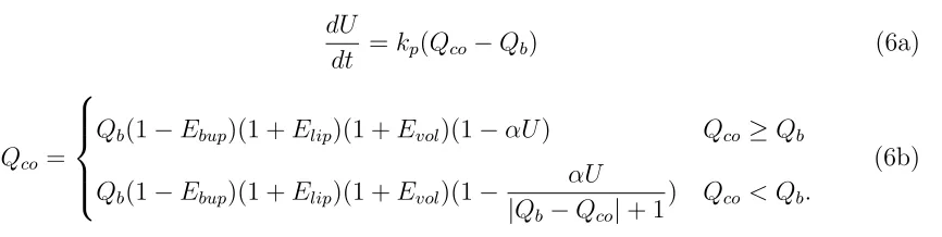
save for one alteration. A modified representation of the homeostatic response (Equations
5a and 5b), was implemented via
dU
dt =kp(Qco−Qb) (6a)
Qco=
Qb(1−Ebup)(1 +Elip)(1 +Evol)(1−αU) Qco ≥Qb
Qb(1−Ebup)(1 +Elip)(1 +Evol)(1−
αU
|Qb−Qco|+ 1
) Qco < Qb.
(6b)
change was introduced because the numerical differential equation solver used for this
study (ode15s.m in MATLAB) requires that solutions be continuously differentiable on
their domain. However, a discontinuity is produced in Equation 5a whenQco approaches
Qb from above. Thus, the conditional aspect of the homeostatic model was transferred
to the equation specifying cardiac output. Note that this was done in such a way as to
ensure continuity in Equation 6b when Qco=Qb. While the optimal values of α and kp
characterizing Equation 6b will differ from those that accomplish likewise for Equation
5b, the behavior originally intended by [14] will be preserved. This fact was verified over
the course of our study.
2.1.3
Inverse Problems
The task of inferring parameter values from data is classified as an inverse problem.
Suppose we have a mathematical model of the form [48]
dy
dt =g(t, y(t), Q) y(t0) = y0.
(7)
This model describes a vector of state variables, y, whose derivative is a function of y,
time, and a parameter set q. In our case, y is 43-dimensional, comprised of the
bupiva-caine concentration, lipid concentration, and total volume in each of the fourteen organ
compartments, as well as Equation 6a. The parameter set Q consists of physiological
parameters (i.e. flow rates, organ volumes, partition coefficients, etc.), which we will
assume to be known, and the the parameters in Table 1 (with, where appropriate, their
pa-state at discrete time points. That is, we have
f(ti, θ0) =h(y(ti), θ0), i= 1, ..., N. (8)
The observable function for this PK/PD model is Equation 6b, which maps the state
vector and parameters of interest to the cardiac output at each of the N = 540 sample
points. Since we cannot assume perfect measurement of the cardiac outputs recorded by
[16], we utilize a statistical model of the form
Yi =f(ti, θ) +Ei. (9)
The random variableEi represents measurement error, which causes discrepancy between
the random variable for the perceived observable state (Yi) and the actual observable state
(f(ti, θ)). We assume that the errors are independently and identically distributed (i.i.d)
with mean ¯E = 0. Realizations of the data correspond to realizations of the random
variables Yi and Ei such that
yi =f(ti,θˆ) +i, (10)
where ˆθ is a parameter set estimating the true parameter set θ0. We obtain ˆθ by
mini-mizing the ordinary least squares (OLS) cost [48]
S(yi, θ) = N X
i=0
[yi−f(ti, θ)]2. (11)
The set ˆθ offering the best approximation of θ0, which lies in the admissable parameter
space Q, is thus [48]
ˆ
θ =argminθ∈Q N X
i=0
An unbiased estimate of the observation variance associated with the estimated vector ˆ
θ, assuming r data points and p parameters, is [48]
ˆ
σ02 ≈ 1
r−p
n X
i=1
[yi−f(ti,θˆ)]2. (13)
Since f(ti, θ) is a function of a system of differential equations, we require numerical
integration software to solve Equation 12. We apply the Matlab function ode15s.m–a
stiff differential equation solver–for this purpose.
Solutions to Equation 12 are generated in two steps. First, in order to avoid becoming
trapped in a local minimum neighboring the literature average values of our parameters of
interest (used as our initial estimates), we perform a Direct search global optimization. In
short, Direct search operates by transforming the problem domain into an N-dimensional
hyper-cube with side length equal to one [17]. The algorithm first determines f(c1),
which is the cost function (Equation 11, in this case) evaluated at the center of the cube.
Next, the costs f(c1 ±δei) are calculated, where δ is one-third the length of the cube
side andei is the unit vector in theith direction. Direct search then establishes a weight
along each direction [17]
wi =min(f(c1+δei), f(c1−δei)), 1≤i≤N. (14)
The region with the minimum wi is divided into thirds. Direct search then identifies
”potentially optimal” regions, divides them as in the initiation step along the longest
dimension, and calculates the corresponding weights wi [17]. This process is repeated
until a global minimum is found as determined by a pre-established tolerance level.
We further refine the parameter estimates obtained through the Direct search by
This function operates using a trust region reflective least squares algorithm, described
in great detail by Coleman and Li [9]. It should be noted that, due to the large range
in magnitudes of the parameter values reported by Fettiplace et al [14], all optimization
steps are performed using log-transformed parameters.
2.1.4
Uncertainty Quantification and Subset Selection
We seek to determine which of the parameters from Table 1 can be reliably estimated
from the data. Reliability, in this context, requires keeping the parameter standard errors
low. To quantify these errors, we estimate all six candidate parameters for each rat. We
then construct a sensitivity matrix, χ, composed of elements
χi,j =
∂Y(ti,θˆ)
∂θˆj
. (15)
That is, the entry in the ith row and jth column is the partial derivative of the model
output (a function of a vector of estimated parameters ˆθ, as before) with respect to the
jthparameter at theith time step [4]. The sensitivity matrix must usually be estimated
numerically, and we elect to do so using the complex step method. This method makes
use of the relationship [4]
∂f
∂x =limh→0
Im[f(x+ih)]
h . (16)
The operator Imrepresents the imaginary component of the specified value. When h is
extremely small (i.e. to machine precision), we can make the approximation [4]
∂f ∂x ≈
Im[f(x+ih)]
h . (17)
ˆ
Σ = ˆσ20[χ(ˆθ)Tχ(ˆθ)]−1. (18)
The model variance ˆσ2
0 is obtained from Equation 13. We obtain an estimate of the
standard error of the kth parameter from the main diagonal of the covariance matrix ˆΣ
according to [48].
SE(ˆθk) = q
ˆ
Σkk. (19)
It is possible that we can drive up parameter standard errors by attempting to fit too
many parameters. To avoid this pitfall, we solve the inverse problem assuming estimation
of all parameters and construct χ. We then take a subset of parameters and construct a
new covariance matrix, ˆΣ0 by taking the columns from χ that correspond to the chosen
parameters and solving Equation 18. We obtain the parameter standard errors for the
subset by applying Equation 19 to ˆΣ0. These standard errors describe a problem in which
the chosen subset is estimated and the other parameters are left constant. We divide the
standard errors by the associated parameter values to obtain normalized standard errors
and compare them to the value 1
1.96. A standard error below this value guarantees that the lower bound of a 95% confidence interval for the associated parameter will be positive.
We repeat this process for every possible parameter subset and choose the combination
that yields the greatest number of parameters with normalized standard errors below the 1
1.96 boundary. For this study, there were
P6 n=1
6
n
= 64 possible parameter subsets.
2.1.5
Time Varying Parameters
We approximate temporal variation in the selected parameters by treating them as
using m linear functions as [44]
P(t) =
p1(t) =a1+b1t t∈[t0, t1)
p2(t) =a2+b2t t∈[t1, t2)
.. .
pm(t) =an+b1t t∈[tm−1, tm]
. (20)
The timest1, t2, ..., tm−1 are the times at which the function changes behavior. By
enforc-ing continuity at these transitions (i.e. p1(t1) =p2(t1), p2(t2) = p3(t2), etc), we create a
spline function. The endpoints of the splines are referred to as nodes, of which there are
m+ 1. Two nodes are external, at p1(t0) and pm(tm), while m−1 nodes occur internally
at p1(t1)...pn−1(tn−1). Spline functions need not be constructed of linear functions, nor
are the nodes required to be evenly spaced across the time domain. However, given the
size of our model, it was computationally sensible to treat them as such.
Representation of a spline function in Matlab can be accomplished by creatingm+ 1
variables corresponding to the function value at each node location. When specified with
a vector of times [t0, t1, . . . , tm], the function interp1.m performs linear interpolation
be-tween the appropriate nodes as dictated by the input time. Spline functions representing
the parameters identified by subset selection are incorporated in the model.
Optimiza-tion requires estimaOptimiza-tion of the node locaOptimiza-tions, growing the parameter set by pm (where
p is the number of parameters selected for time variation). To characterize the trade-off
between model performance and computational efficiency, we investigate spline
approx-imations of m = 1, m = 4, and m = 8 in the time-varying models. We select these
values so that splines can be progressively nested each time m is increased, allowing us
2.1.6
Model Selection
Model selection seeks to extract from a candidate pool a single model that provides the
best fit to the data while avoiding unnecessary complexity and overfitting. Referred to
as the ”Principle of Parsimony”, this balance is determined by the number of parameters
estimated [25]. Too few parameters will result in a biased model, while too many will drive
up the variance and make the model unreliable for out-of-sample predictive purposes. One
method of quantifying the appropriateness of a model is to apply the Akaike Information
Criterion [48]
AIC =rln(Smin
r ) +r(1 +ln(2π)) + 2(p+ 1). (21)
The variablesrandprefer to the number of sample points and the number of parameters
in the model, respectively. Smin is the minimum value of Equation 11 achieved by
apply-ing the parameters satisfyapply-ing Equation 12. Models with lower AIC scores are considered
to be the most appropriate for the data in question.
A drawback to relying solely upon AIC is that the difference between two scores does
not directly translate to a statement of statistical significance. We therefore supplement
our model selection procedure with model comparison nested restraint tests. Nested
restraint tests assume two models with parameter estimates ˆθ and ˆθN belonging to
re-spective admissible spacesQandQN, withQN ⊂Q[48]. That is, the estimates in ˆθN are
a subset of the estimates in ˆθ. We desire to know whether the true parameterθ0 is in the
subset QH; therefore we test the null hypothesis H0 : θ0 ∈ QN, against the alternative
HA:θ0 ∈ Q[48]. If we denote Smin and S
(N)
min as the minimum OLS costs corresponding to ˆθ and ˆθN (solutions of Equation 12), then clearly Smin ≤ S
(N)
points, we can thus define a test statistic [48]
T = r(S
(N)
min−Smin)
Smin
. (22)
The statistic T can be compared to a χ2 distribution with degrees of freedom equal
to the difference in the number of parameters contained in ˆθ and ˆθN. These tests will
be utilized in conjunction with AIC scores to determine which parameters identified by
subset selection should be treated as time varying and to establish the number of splines
sufficient to represent them.
2.2
Results
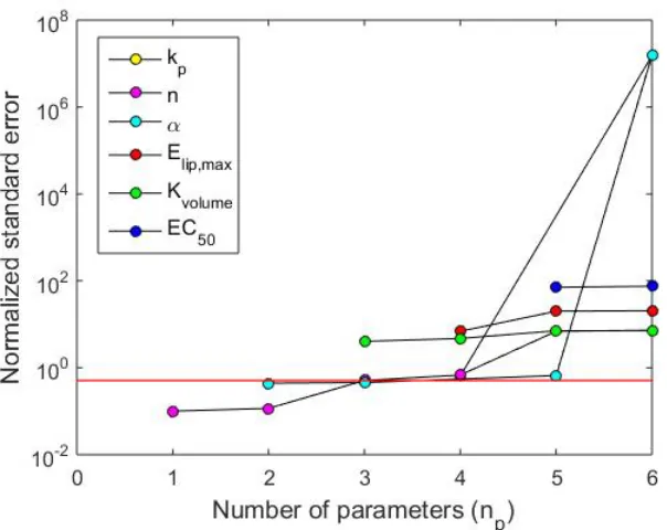
The results of subset selection for one of the subjects are presented in Figure 2. We
note that, across all subjects, the consistent consensus was thatn and one of the control
parameters (eitherαorkp) should be estimated. Since analysis of the off-diagonal entries
of the covariance matrices demonstrated α and kp to be perfectly correlated, the choice
between the two was inconsequential and we arbitrarily selectedα. Spline representations
ofnandαwere thus incorporated in the PK/PD model for estimation and the remaining
parameters in Table 1 were set to their population averages and not estimated. We
hereafter refer to our candidate models as Constant, mn, mα, and mn/α, where m
represents the number of splines used to describe time variance (either 1, 4, or 8) and n,
α, and n/α denote which parameters are selected for time variance.
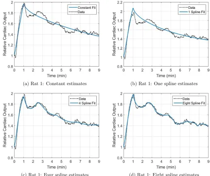
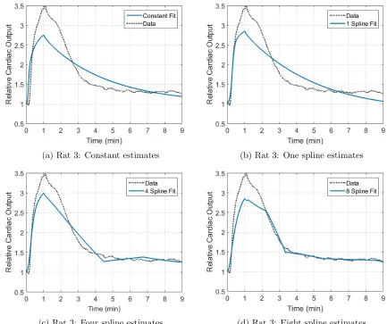
The corresponding model fits for m = 0, 1, 4, and 8 splines are presented in Figures
3-9, in which both n and α are assumed to be time variant. We should note that the
number of splines used for n and α are always equal (that is, for instance, there is no
cases, a simulated dose of 9 mL/kg of Intralipid is injected at a constant rate for 1 minute
starting at time t = 0. We then compare the one, four, and eight spline functions for n
and α across all subjects to establish potential population trends (Figures 10-11).
Akaike Information Criterion (AIC) scores are tracked across all parameter and spline
combinations for each subject in Figures 12-13. Figure 14 summarizes how growing the
number of splines affects AIC scores of all subjects with respect to the model in which
n and α both vary (which was clearly superior to the other models). Finally, we present
the distributions of n and α at each node location for the four spline model (Figure
15) to motivate our choice of probability function from which to sample for our virtual
population study.
Figure 2: Subset selection results for candidate parameters for estimation. Red line denotes a normalized
standard error less than 1
(a) Rat 1: Constant estimates (b) Rat 1: One spline estimates
(c) Rat 1: Four spline estimates (d) Rat 1: Eight spline estimates
(a) Rat 2: Constant estimates (b) Rat 2: One spline estimates
(c) Rat 2: Four spline estimates (d) Rat 2: Eight spline estimates
(a) Rat 3: Constant estimates (b) Rat 3: One spline estimates
(c) Rat 3: Four spline estimates (d) Rat 3: Eight spline estimates
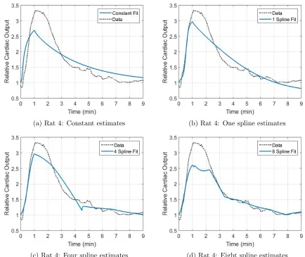
(a) Rat 4: Constant estimates (b) Rat 4: One spline estimates
(c) Rat 4: Four spline estimates (d) Rat 4: Eight spline estimates
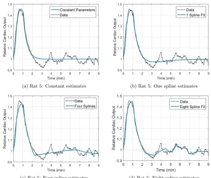
(a) Rat 5: Constant estimates (b) Rat 5: One spline estimates
(c) Rat 5: Four spline estimates (d) Rat 5: Eight spline estimates
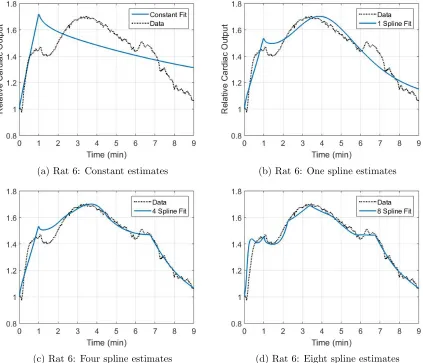
(a) Rat 6: Constant estimates (b) Rat 6: One spline estimates
(c) Rat 6: Four spline estimates (d) Rat 6: Eight spline estimates
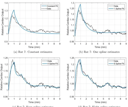
(a) Rat 7: Constant estimates (b) Rat 7: One spline estimates
(c) Rat 7: Four spline estimates (d) Rat 7: Eight spline estimates
(a) m = 1 (b) m = 4
(c) m = 8
(a) m = 1 (b) m = 4
(c) m = 8
(a) Rat 1: AIC Scores (b) Rat 2: AIC Scores
(c) Rat 3: AIC Scores (d) Rat 4: AIC Scores
Figure 12: AIC Scores for Subjects 1-4 across models with time variation in combinations of n andα
(a) Rat 5: AIC Scores (b) Rat 6: AIC Scores
(c) Rat 7: AIC Scores
Figure 13: AIC Scores for Subjects 5-7 across models with time variation in combinations of n andα
Figure 14: AIC Scores for all subjects using spline representations for n and α as a function of the number of splines Used. The models using four and eight splines produce very similarly appropriate fits for many of the subjects
Table 2: P-values for nested model comparison tests for each rat. In each test, the first model listed is nested within the second, and a p-value of less than 0.05 indicates that the second model is significantly improved over the first. The model with four-spline representations of both n and α is significantly superior to the constant model (Test 6), the one-spline models (Tests 7-9), and the four-spline models with either nor α time varying (Tests 10-11). Introduction of eight-spline representations ofn andα
does not offer significant improvement for 4 of the 7 rats (Test 12)
Model Test Rat 1 Rat 2 Rat 3 Rat 4 Rat 5 Rat 6 Rat 7
1) Constant vs 1n 1.000 0.000 0.000 0.000 0.000 0.000 0.000
2) Constant vs 1α 1.000 0.000 0.046 0.000 0.000 0.000 0.000
3) Constant vs 1n/α 1.000 0.000 0.000 0.000 0.000 0.000 0.000
4) Constant vs 4n 1.000 0.000 1.000 0.000 0.000 0.000 0.042
5) Constant vs 4α 0.000 0.000 1.000 0.000 0.000 1.000 0.000
6) Constant vs 4n/α 0.000 0.000 0.000 0.000 0.000 0.000 0.000
7) 1n vs 4n/α 0.000 0.000 0.000 0.000 1.85 x 10⁻¹¹ 0.000 0.000
8) 1α vs 4n/α 0.000 0.000 0.000 0.000 0.000 0.000 0.000
9) 1n/α vs 4n/α 0.000 0.000 0.000 0.000 0.000 0.000 0.000
10) 4n vs 4n/α 0.000 1.000 0.000 0.000 1.23 x 10⁻⁷ 0.000 0.000
11) 4α vs 4n/α 0.000 5.48 x 10⁻¹⁴ 0.000 0.000 1.02 x 10⁻⁸ 0.000 1.00
(a) Parameter: n
(b) Paramater: α
Figure 15: Distributions of estimated node locations for four-spline representations of (a) nand (b)α
2.3
Discussion
The results of subset selection, which were previously mentioned, indicate that we do
not possess sufficient information to estimate all six parameters listed in Table 1 with
reasonable confidence. Of the three parameters we did not estimate (excludingkp, which
is perfectly correlated with α), two contribute to the Hill equation for lipid dynamics
(EC50 and Elip,max in Equation 3), and the third describes the flow promoting effect of
increasing the volume in the bloodstream (Kvolume in Equation 4). In retrospect, it is not
surprising that we could not estimateKvolume because without a control we cannot isolate
the volume effect from the inotropic effect of the lipid. The same study by Fettiplace et
al [16] from which we obtained lipid infusion data utilized a saline control infusion, but
we did not have access to this data on an individual subject level. Likewise, estimation
of Elip,max and EC50 would be more feasible if our data had included multiple trials for
each subject.
While unfortunate, these restrictions did not prevent us from achieving good fits
via estimation of n and α. Akaike Information Criteria (AIC) scoring clearly indicates
preference for the n/α models over the the Constant, n, and α models. (Figures 12-13).
The results of the model comparison tests (Table 2) are consistent in this regard. Table 2
shows that the one-spline models are not consistently preferable to the constant estimate
models, but that the 4n/α model is significantly better than all constant and one-spline
models. The exception noted by both AIC and model comparison is Rat 7 (Figure 13c
and Test 11 in Table 2), for which the 4α model provides the best fit. This outcome is
likely due to the low peak (max ≈ 1.23 at 0.75 minutes) in cardiac output experienced
by Rat 7 (Figure 9). We might postulate therefore that n is the more critical parameter
The flexibility conferred by the utilization of linear splines is apparent in Figures 3-9.
Assumption of constant parameter estimates allows the model to fit relatively smooth
responses with a single peak (Figures 3a and 7a), but irregular dynamics such as those
exhibited in Figure 4a and 8a cannot be captured. The addition of a single spline
rep-resentation significantly improves the tracking ability of the model, as Figures 4b and
8b attest. Even with time varying parameters, though, the model has difficulty fitting
large initial peaks in relative cardiac output such as those experienced by Rats 3 and 4
(Figures 5 and 6). This limitation could be due to relying upon a population estimate
for Elip,max (the parameter capturing the maximum effect of the lipid), rather than
in-dividual estimates. Including more splines does not resolve this issue, but it does allow
the model to better detect sustained oscillations in the data (Figures 3, 7, and 9).
Of course, oscillation tracking may not be a desirable trait, as it is possible that the
model is fitting noise rather than biologically relevant information. The spline
represen-tations ofn and α in Figures 10 and 11 can shed light on this matter. Ideally, we would
prefer that the process of least squares estimation has not over-fit the data such that
physiologically unreasonable or spuriously oscillatory parameter values are introduced.
The first of those pitfalls does not appear to be an issue, as the respective estimates of n
and α at each node location (for all spline cases) are on the same order of magnitude as
each other and as the population estimates reported by Fettiplace et al [14]. However,
increasing the number of splines from four to eight introduces potentially meaningless
(and large) oscillations in n (Figures 10b and 10c). This trend is particularly apparent
with respect to Rats 3 and 4, which we previously noted had large initial peaks in cardiac
output. It is likely, therefore, that the spline approximation is estimating large and fast
changes inn in an unsuccessful attempt to model these peaks. The fact thatn is singled
with greater influence on the magnitude of response.
The parameter α, conversely, does not display biologically unreasonable behavior
as the number of splines is increased from one to eight. The four and eight spline
cases demonstrate ideal behavior in that the time varying parameters drift initially but
converge towards what appear to be constant, baseline values (Figures 11b-11c). Rats
5 and 7, which had relatively lower estimates for n, demonstrated the largest α values
compared to the other subjects. These two rats differ from the others in that they exhibit
the two lowest initial peaks in relative cardiac output as well as sustained oscillations
in cardiac activity throughout the time domain (Figures 7 and 9). The value of α,
therefore, could be the more important parameter with respect to the smoothness (or
lack thereof) of cardiac response to lipid infusion. Though an eight-spline representation
of α qualitatively appears reasonable, an equivalent representation of n is not, likely
making an eight spline model untenable.
Analyzing results from AIC and model comparison tests leads us along a similar
chain of logic. Figure 14 confirms that introducing four-spline representations of α and
n consistently improves model performance over constant estimate and one-spline fits.
However, doubling the number of splines from 4 to 8 results in a poorer model in four
cases. Two of these instances follow from the model being unable to fit the maximum
cardiac outputs experienced by Rats 3 and 4 (Figures 5-6), as discussed previously. Since
the increase in model complexity does nothing to improve the fit, no reduction in AIC is
accomplished. AIC scores also increased from the four-spline model to the eight-spline
model for Rats 6 and 7, indicating that, though the fit visually appears improved, we
over-fit the data in these two cases and do not capture meaningful information. The
comparison test 12 in Table 2 identifies the same four rats as experiencing no significant
In consideration of these factors, the 4n/α model represents the most appropriate
choice for our study. Allowing time variation in n and α renders the model capable
of predicting dynamic individual responses to lipid emulsion infusion. By restricting the
number of splines used for time variance, we achieve good fits to the available data without
over-fitting or introducing unreasonable values or oscillations in our biological parameters.
The process of model testing also provided insight as to the potential physiological roles
of each parameter, with n dictating the magnitude and shape of response and α serving
as a smoothing factor.
3
Parameter Estimation 2
3.1
Methods
We recall that the results obtained above were constrained by insisting that splines be of
equal length. That is, for example, a two-spline function for n was composed of one line
defined on the time interval [0,4.5] and another defined on [4.5,9]. If we revisit Figures
10b and 11b, though, we see that neither parameter changes consistently across the time
domain. The parameter α undergoes noticeable changes over the first 2 minutes but
remains comparably constant over the final 7 minutes for all subjects. Likewise, each rat
shows a contrast in the behavior ofn before and after 4 minutes.
We therefore desire to test if we can reduce the number of parameters in our model–
while maintaining our model performance–by more judiciously selecting the node
loca-tions for each spline function. We introduce to our model a time vector [0,2,9] containing
the node locations for α and a time vector [0,4,9] containing the node locations for n
(each node represents a time in minutes). Each parameter is thus described by two splines
3.2
Results
The model fits attained using unique two-spline representations of n and α (denoted
2∗n/α henceforth) are presented in Figures 16-22. For the purpose of comparison, the
1n/α and 4n/α fits are presented with each of the 2∗n/α fits. We then calculate the
AIC score associated with each new model and plot it along with the original models
in Figures 23-24. Since the node locations are no longer consistent for all parameters,
we cannot perform model comparison nested restraint tests. Thus, our sole quantitative
(a) Rat 1: m = 2* Splines
(b) Rat 1: m = 1 spline (c) Rat 1: m = 4 splines
(a) Rat 2: m = 2* Splines
(b) Rat 2: m = 1 spline (c) Rat 2: m = 4 splines
(a) Rat 3: m = 2* Splines
(b) Rat 3: m = 1 spline (c) Rat 3: m = 4 splines
(a) Rat 4: m = 2* Splines
(b) Rat 4: m = 1 spline (c) Rat 4: m = 4 splines
(a) Rat 5: m = 2* Splines
(b) Rat 5: m = 1 spline (c) Rat 5: m = 4 splines
(a) Rat 6: m = 2* Splines
(b) Rat 6: m = 1 spline (c) Rat 6: m = 4 splines
(a) Rat 7: m = 2* Splines
(b) Rat 7: m = 1 spline (c) Rat 7: m = 4 splines
(a) Rat 1: Updated AIC Scores (b) Rat 2: Updated AIC Scores
(c) Rat 3: Updated AIC Scores (d) Rat 4: Updated AIC Scores
Figure 23: AIC Scores for Subjects 1-4 across models with time variation in combinations of n andα
(a) Rat 5: Updated AIC Scores (b) Rat 6: Updated AIC Scores
(c) Rat 7: Updated AIC Scores
Figure 24: AIC Scores for Subjects 5-7 across models with time variation in combinations of n andα
3.3
Discussion
The 2∗n/α provides an interesting compromise between the 1n/α and 4n/αmodels. One
shortcoming of the 4n/α model is that, in some instances, the node placement causes
the model to mistime a peak in cardiac output (see Figures 16c, 20c, 21c, and 22c). The
analogous 2∗n/α models (Figures 16a, 20a, 21a, and 22a) more accurately capture both
the height of the maximums and the times at which they occur, which is a desirable trait.
At the same time, the new model avoids the overshoot that is occasionally an issue with
the 1n/α models (Figures 16b and 22b) while preserving the ability to cut through the
mean values of oscillatory regions rather than trying to track them exactly. This aspect
may or may not be desirable, depending on the biological significance of those regions.
According to the weights assigned by AIC to these relative strengths and weaknesses,
the 2∗n/α model is not preferable to the 4n/α model. The 2∗n/α model, however, is
useful to consider in future modeling efforts, particularly as we gain access to more data.
If we are able to estimate more parameters, removing some of the data fitting burden
fromnand α, two carefully placed splines could prove sufficient to produce a model with
high accuracy. Additionally, with only seven subjects, we do not have a firm grasp on
what a typical response looks like. We might learn after collecting more data that we
should not be overly concerned with the oscillations in cardiac output exhibited by some
subjects. In such an event, the 2∗n/α model would likely be the best choice. Since we
are limited, though, to the information presently available, we will use the 4n/α model
4
Virtual Population Studies
4.1
Methods
Based on the distributions of estimates for n and α for our selected model (Figure 15),
we elect to designate our parameters as belonging to log-normally distributed functions.
We make this choice given that most of the box plots are right-skewed, particularly in
the case ofα. The log-normal distribution is given by
X =eµ+σz (23)
Here, X is a random variable whose natural logarithm has a normal distribution
centered at µ with standard deviation σ (z is the standard normal variable)[40]. The
expected value and variance ofX are [40]
E(X) = eµ+
1 2σ
2
(24a)
V ar(X) =e2(µ+σ2)−e2µ+σ2 (24b)
We estimate the values µ and σ–which are sufficient to define a given distribution–for
each parameter using the Matlab function lognfit.m.
Using these distributions, we construct virtual populations of rats undergoing two
different ILE therapy regimens in response to LAST induced by intravenous absorption
of bupivacaine. Bupivacaine overdose is modeled as a 10 mg/kg infusion administered at
a constant rate for 20 seconds. Treatment with lipid is assumed to begin 10 seconds after
completion of bupivacaine infusion. The two treatment regimens consist of 4 mg/kg of
![Figure 1: Physiologically Based Compartmental Pharmacokinetic Model for Bupivacaine [29]](https://thumb-us.123doks.com/thumbv2/123dok_us/1273093.1159861/23.612.214.417.73.324/figure-physiologically-based-compartmental-pharmacokinetic-model-bupivacaine.webp)