Assessment of Structural Properties Based on Measured Acceleration Data by
System Identification Scheme
Inho Yeo l), Joo Sung Kang 2), Jeong-Moon Seo 3) and Hae Sung Lee 2) 1) Highway Management Corporation, Research Institute, Ichon, Korea
2) School of Civil, Urban and Geosystem Engineering, Seoul National University, Seoul, Korea 3) Korea Atomic Energy Research Institute, Daejon, Korea
ABSTRACT
This paper introduces an algorithm for the parameter estimation scheme based on the system identification in time domain. In this study, acceleration data by a dynamic test are used as the measured responses. The least squared errors of the difference between calculated acceleration and measured acceleration are adopted as an error function. Tikhonov regu- larization technique is applied to alleviate the ill-posedness of the inverse problem in the system identification (SI). The regularization factor is determined by the geometric mean scheme (GMS). The recursive quadratic programming (RQP) is adopted to solve the constrained nonlinear optimization problem of the least squared errors. First order of sensitivity of ac- celeration is obtained by direct differentiation of the equation of motion. The validity of the proposed method is demo n- strated by numerical examples.
I N T R O D U C T I O N
The modal analysis approaches have been widely adopted to identify structural properties using measured accelera- tion. The modal analysis approaches suffer from drawbacks caused by insensitiveness of modal data to changes of struc- tural properties. In addition, the damping properties of structures cannot be estimated by the modal analysis. To overcome the drawbacks of the modal analysis approaches, this paper presents a system identification scheme to determine structural properties such as stiffness and damping parameters of structures using measured acceleration data. The proposed algorithm is based on the minimization of an error function with respect to the structural parameters. The error function is defined as the time integral of the least squared errors between the measured acceleration and the calculated acceleration by a mathe- matical model.
A system identification problem is a type of inverse problem, which is usually ill-posed. An ill-posed problem is characterized by the non-uniqueness and instability of solutions. The regularization technique has been employed to over- come the ill-posedness of inverse heat transfer problems and inverse elasticity problems. In the regularization technique, a predefined regularization function is added to the error function to impose constraints on the admissible solutions of a given inverse problem. This paper introduces a new regularization function that is defined as the L2 norm of the time derivative of system parameters. To determine the regularization factor, which has crucial effect on the solution of the SI scheme, the geometric mean scheme is adopted.
The validity and effectiveness of the proposed method will be demonstrated with several numerical examples. The numerically generated data with noise are utilized as measured acceleration. Detailed discussions on the numerical behav- iors of the proposed method are presented.
PARAMETER ESTIMATION SCHEME IN TIME DOMAIN
The unknown system parameters of a structure including stiffness and damping properties are identified by minimizing least squared errors between computed and measured acceleration at some discrete observation points.
t
if
FIE (t) = Min -~ d, subject to R (x) < 0 0
(1)
where ~ , [ , x and R are the calculated acceleration and the measured acceleration at time t, system parameter vector and constraint vector, respectively, with IIII representing the Euclidean norm of a vector. Linear constraints are used t o s e t physically significant upper and lower bounds of the system parameters. The minimization problem defined in Eq. (1) is a constrained nonlinear optimization problem because the acceleration vector ~ is a nonlinear implicit function of the system parameters x.
:! ._~i ii~ { ~ ~ !
SMiRT 16, Washington DC, August 2001 Paper # 1805
The parameter estimation defined by a minimization problem as Eq. (1) is a type of ill-posed inverse problems. Ill- posed problems suffer from three instabilities: nonexistence of solution, non-uniqueness of solution and discontinuity of solu- tions when measured data are polluted by noises. Because of the instabilities, the optimization problem given in Eq. (1) may yield meaningless solutions or diverge in optimization process. Attempts have been made to overcome instabilities of inverse problems merely by imposing upper and lower limits on the system parameters. However, it has been demonstrated by several researchers that the constraints on the system parameters are not sufficient to guarantee physically meaningful and numerically stable solutions of inverse problems [ 1,2].
The regularization technique proposed by Tikhonov is considered as a more rigorous way to overcome the ill- posedness of inverse problems. In the regularization technique, the original object function is modified by adding a positive definite regularization function [3,4]. Various regularization functions are used for different types of inverse problems. The following regularization function is adopted for the parameter estimation in time domain.
nR(t)=~.
&
(2)
where ~, is the regularization factor. The regularization function defined in Eq. (2) represents the variance of system pa- rameters in time. By adding the regularization function to the error function, the regularized parameter estimation scheme is defined as follows.
ill
Minx H(t) = a ( x ) - 2 d t + ~ dt
0
0
subject to R (x) < 0 (3)
The regularization function in Eq. (3) enforces the system parameters to vary smoothly in time, and thus enhances the uniqueness and continuity of the system identification problems by preventing the system parameters from arbitrary changes. Since the solution space of the system identification problem is restricted by the regularization function during optimization, the upper bounds of system parameters do not have to be set near the baseline properties of the system parameters.
The regularization effect in parameter estimation process is determined by the regularization factor. The regulariza- tion effect vanishes for a small regularization factor while the regularization function has a dominant effect over the error function during the optimization process for a large regularization factor. In either case, the optimization problem is unable to estimate correct system parameters due to instabilities or excessive regularization effects on the system parameters. Therefore, selection of a proper regularization factor is very crucial to obtain meaningful solutions of system identification problems. The geometric mean scheme proposed (GMS) by Park is adopted in this study to determine the optimal regulafi- zation factor [5]. In the GMS, the optimal regularization factor is defined as the geometric mean between the maximum singular value and the minimum singular value of the Gauss-Newton hessian matrix of the discretized error function given in Eq. (1).
~op,
=4Smax "Smin
(4)where
~,opt,
Smax, Smin
denote regularization factor, maximum singular value and minimum singular value which is greater than zero, respectively. The singular values of any given matrix can be obtained by using the singular value decom- position [6]. The discretized form of the error function will be presented in the next section.DAMPING MODEL
It is a difficult task to model damping properties of real structures. In fact, existing damping models cannot de- scribe actual damping characteristics exactly, and are approximations of real damping phenomena to some extents. Since the damping has an important effect on dynamic responses of a structure, the damping properties should be considered prop- erly in the parameter estimation scheme. In most of previous studies on the parameter estimation, the damping properties of a structure are assumed as known properties, and only stiffness properties are identified. However, the damping properties are not known a priori and should be included in system parameters in the SI.
C = M( n~~ 2(nOgn ~"Onr ~ M .
(5)
where M, N, Mn, ~n, ~ and tth denote mass matrix, the number of the degrees of freedom (DOF), n-th generalized modal mass, modal damping ratio for n-th mode, the n-th mode shape and n-th mode frequency, respectively. In Rayleigh damping, a damping matrix is represented by a linear combination of the mass matrix M and stiffness matrix K.
C = a 0 M + alK (6)
The damping coefficients of the Rayleigh damping can be determined when any two modal damping ratios and the corre- sponding modal frequencies are specified.
In ease the modal damping is employed in the parameter estimation, the number of the system parameters associated with the damping is equal to that of the total number of DOFs, which increases the total number of unknowns in the optimiza- tion problem given in Eq. (3). Since neither modal damping nor Rayleigh damping can describe actual damping exactly, and the modal damping requires more unknowns than the Rayleigh damping in the parameter estimation, this study employs the Rayleigh damping for the SI. The Rayle igh damping yields a linear fit to the exact damping of a structure.
TIME D I S C R E T I Z A T I O N AND SENSTIVITY
The object function in Eq. (3) is easily discretized with respect to time as follows
= 1 i
0
0
1 ~11~, ~,11 ~ +_~ ~ II x'-~,x''ll ~
= - - - At --"
2 k=~ 2 k=~
n t
2 ~ l l
At II
IEII~ ~ll=
~
x~-x ~-'~
4
= - - At + - -
2 k=l k=l
~ IIxn,_xn, ill 2
2 At
(7)
where the superscript denotes time step and nt represents the current time step, i.e., t = n t x A t . Since the system parame- ters of former time steps are known, and have no effect on the solution of the minimization problem, the second term of the last equation in Eq. (7) can be omitted from the object function.
_ kll 2
.~t.= 7 II ~k
~ , +k=l
~ IIxn,_xn, ill 2
2 At
(8)
The Newmark 13 method is employed to obtain the acceleration at each time step. The equation of motion of a structure is
Ma + Cv + Ku = p(t) (9)
where u, v and p(t) are displacement, velocity and an external excitation force, respectively. The increments of the dis- placement, velocity and acceleration at (i+ 1)-th time step are given as
Y " Y v - A t ( l - " ? ' ~
~v, = ~ Z ; ~ . , - g
,
g
i
1 1 1
~x~i = (13,~,)---z-,~. i - - ~ v , - N a ~
where 13 and 7 are the integration constants of the Newmark 13 methods, and
Api = Ap i + (~At M "l- )Vi + ('~" M + At C)ai
1
I ( = K + Y C + M
~ A t ~ ( A t ) 2
(11)
where Au i, Avi andAa~ are the increments of displacement, velocity and acceleration, respectively The total displacement, velocity and acceleration at the (i+l)-th time step are calculated as follows.
Ili+ 1 = U i q - A u i Vi+ 1 - V i d - A v i
a i+ 1 = a i + A a i
(12)
The recursive quadratic programming with Fletcher active set strategy is utilized to perform the optimization of Eq. (8). The line search is employed to accelerate convergence of the optimization. The sensitivity of the acceleration with respect to the system parameters is obtained by the direct differentiation of Eq. (10)-(12).
E X A M P L E
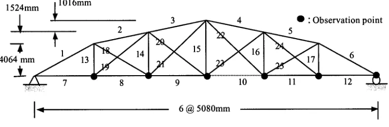
The validity of the proposed time domain SI is examined through a simulation study with a bowstring truss shown in Fig. 1. The bowsting truss consists of 12 nodes and 25 members. The axial stiffness and the weight per unit length of each member (top member, bottom member, vertical member and diagonal member) are given in Table 1. t is assumed that the cross- sectional area of the 10 th bottom member is reduced by 33% from its original value. For the numerical simulation study, the measured responses is obtained by a free vibration induced by the initial displacement. The initial displacement is taken as the displacement caused by the vertical unit load on the lower center of the structure in static equilibrium. Newmark 13 method is used to obtain the acceleration data. The damping of the real structure is assumed as the modal damping. The acceleration is measured in the time period from 0 see to 8 see with the interval of 1/16 sec.
1524mm ~1016mm
3 4 Q • Observation
~ point
- I
/ ~ 7 8 9 10 11 12 ~
.._1
I 6 @ 5080mm v[
Fig. 1. The geometry shape of truss structure
Table 1. Material property of bowstring truss
Member Top member Bottom member
Mass per unit length
(K~/m)
62.40
Axial stiffness property(EA)
1.680e+04
50.70 1.365e+04
Vertical member 32.76 1.131 e+04
C a s e 1 : w i t h o u t d a m p i n g e s t i m a t i o n a n d m e a s u r e m e n t e r r o r
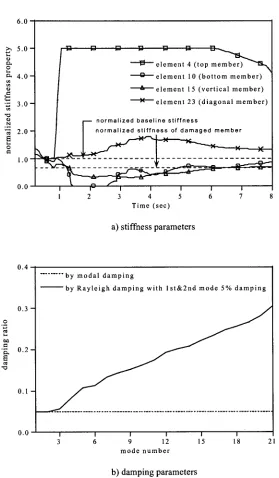
The parameter estirmtion is performed without damping estimation. Measurement errors are not taken into account to dem- onstrate the effect of damping in the parameter estimation. The measured acceleration data are obtained by the 5% modal damping, while the Rayleigh damping is employed in the SI. The coefficients of the Rayleigh damping are calculated by the first two modal damping coefficients and the corresponding frequencies, and are fixed through the parameter estimation. Fig 2a shows identification results of the stiffness parameters. Although no measurement error is presented, the identifica- tion results exhibit extreme instabilities. None of stiffness property converges to a correct value. This is because the damping characteristics cannot be adjusted to represent measured accelerations. As shown in Fig.2b, there exists big dis- crepancy between real modal damping and the Rayleigh damping used in SI.
I ~ element 15 (vertical member)
;~ 5 . 0 -
o ~ 4 . 0 -
• ~ 3.0 r~
6.0
o
.N [---- normalized b a s e l i n e s t i f f n e s s
2.0
o 1.0
0 . 0 I I I I .... I " "-'1 - "==- - [
1 2 3 4 5 6 7 8
Time (sec)
a) stiffness parameters
0.4
0 , 3 -
O .,-q 0= eL0 • ~, 0 . 2 -
E "o
0 . | --
... by modal damping
" - - " - - b y Rayleigh damping with l st&2nd mode 5% damping
0.0
J
/
/
/
I I I I I I
3 6 9 12 15 18 2
mode number
b) damping parameters
1.6 ] ~ e l e m e n t 4 (top m e m b e r )
;~ 1.4 4 -~ element 10 ( b o t t o m m e m b e r )
] d i a g o n a l m e m b e r )
o
" x element 15 ( v e r t i c a l m e m b e r )
o ~ 1 . 2
",~, 1 " 0 ~ - £ " . . . . -- .. . . ~____~_ __ A
CD
,.~ 0.8 1 ~ ~ n o m a l i z e d b a s e l i n e s t i f f n e s s
o
i= 0.6 f
t
~ ~
...
normalized
s t i f f n e s s of d a m a g e d m e m b e r0.4
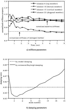
In this case, the coefficients of the Rayleigh damping are included in the parameter estimation. To demonstrate the effect of the damping estimation, measurement error is not considered. As shown in Fig. 3a, the stiffness properties con- verges to the exact values of the corresponding members. The identification results of the damping coefficients are shown in Fig. 3b. The estimated coefficients of the Rayleigh damping approximate the real modal damping by a linear fit. It is clearly understandable that the accuracy and stability in the parameter estimation are gained by the damping estimation.
I I I I I I I
1 2 3 4 5 6 7 8
Time ( s e c )
a) stiffness parameters
0.10 ] ... by m o d a l d a m p i n g
0.09 1 by e s t i m a t e d R a y l e i g h d a m p i n g
0.08
o .,..~
" 0 . 0 7 - eLO I=
0 . 0 6 -
0.05 -
0.04 -
0.03 I I I I I I
3 6 9 12 15 18 21
m o d e n u m b e r
Case 2 : with damping estimation and no measurement error
b) damping parameters
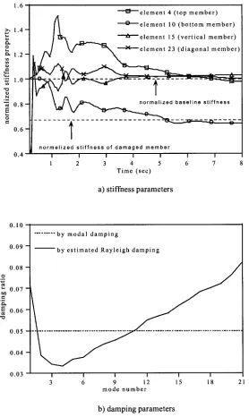
C a s e 3 : with d a m p i n g e s t i m a t i o n a n d m e a s u r e m e n t e r r o r s
The parameter estimation is performed with damping estimation and measurement errors to examine the effect of measure- ment errors on the parameter estimation. To simulate measurement errors, 5% proportional errors are added to the calcu- lated acceleration. As shown in Fig. 4a, there exist slight instabilities for the stiffness parameter estimation in early time step until around 3see. Nevertheless the estimated values of the system parameters stay in reasonable region by the effect of the regularization function. The estimated values of stiffness parameters converge to exact value after about 5 see. The estimated damping coeffic ients are little influenced by the measurement errors.
1.6
"~" e l e m e n t 4 (top m e m b e r )
~, 1.4
O
o 1.2
r~ ID
"~ 1.0
O
0.8
0
e l e m e n t 10 ( b o t t o m m e m b e r )
• ~ e l e m e n t 15 ( v e r t i c a l m e m b e r )
e l e m e n t 23 ( d i a g o n a l m e m b e r )
1~ "" ~ ' ~ " 1
n o r m a l i z e d b a s e l i n e s t i f f n e s s
061 l
- ' - "n o r m a l i z e d s t i f f n e s s o f d a m a g e d m e m b e r
0.4 i i I I I
1 2 3 4 5
I I
6 7 8
Time (sec)
a) stiffness parameters
0.10 / . . . by m o d a l d a m p i n g
0.09 1 by e s t i m a t e d R a y l e i g h d a m p i n g
0.08 .R
0.07
,~ 0.06
0.05
0.04
0.03 i I I I I i
3 6 9 12 15 18 2
m o d e n u m b e r
b) damping parameters
C O N C L U S I O N
A time domain SI using measured acceleration data is proposed. The least squared error of the difference between calculated acceleration and measured acceleration is adopted as an error function. The Tikhonov regularization technique is employed to alleviate the ill-posedness of the inverse problem in SI. The GMS is utilized to determine the optimal regulafi- zation factor. The Rayleigh damping is used to estimate the damping characteristics of a structures. The system parame- ters include the damping coefficients of the Rayleigh damping as well as the stiffness parameters of a structures.
In most previous study, the damping characteristics of a structure are assumed as known values. It is confirmed that severe instabilities can be occurred by incorrect assumption of damping matrix and that the damping characteristics should be adjusted properly according to measured acceleration data. It is not possible to form the exact damping matrix of a structure, but it is very important to approximate the damping matrix to the real damping matrix as close as possible. The proposed method can estimate the stiffness properties accurately even though the damping characteristics are approximated by the Rayleigh damping. When the measured data are polluted by noises, the convergence rate becomes a little slow. However, the final solution converges to the exact solution even for noise-polluted data. It is believed the proposed method provides a very powerful engineering tool to identify dynamic characteristics of structures and to detect damage in structures based on measured acceleration.
R E F E R E N C E S
1.Hjelmstad, K.D., "On the uniqueness of modal parameter estimation," Joumal of Sounds and Vibration, Vol. 192(2), 1996, pp. 581-598.
2.Neuman, S.P., and Yakowitz, S., "A statistical approach to the inverse problem of aquifer Hydrology," Water Resources Research, Vol. 15(4), 1979, pp. 845-860.
3.Bui, H.D., Inverse problems in the mechanics of materials: An introduction, CRC Press, Boca Raton, 1994.
4.Hansen, P.C., Rank-deficient and Discrete Ill-Posed Problems: Numerical Aspects of Linear Inversion .SIAM: Philadel- phia, 1998.
5.Park, H.W., Shin, S.B. and Lee, H.S., "Determination of Optimal Regularization Factor for System Identification of Lin- ear Elastic Continua with the Tikhonov Function," Intemational Journal for Numerical Methods in Engineering, Vol. 51, No.10, 2001, pp. 1211-1230.
6.Golub, G.H. and Van Loan C.F., Matrix Computations (3rd edition). The Johns Hopkins University Press: London, 1996. 7.Chopra A.K., Dynamics of Structures (theory and applications to earthquake engineering), Prentice Hall, 1995.