ABSTRACT
HU, SHUMING. Approximations and Effectiveness of QMC and Other Electronic Structure Methods in Molecules and Solids. (Under the direction of Lubos Mitas.)
Accompanying the development of methodologies and computer technology,
first-principle electronic structure calculations are gaining a stronger foothold as well as wider
applicability in predicting material properties. We examined and compared fundamental
approximations made in different electronic structure methods like Hartree-Fock (HF),
Density Functional Theory (DFT) and quantum Monte Carlo (QMC). Some of their
boundaries and effectiveness are analyzed through both simple systems as well as real
world materials.
Thorium monoxide’s energy and electric properties were studied using HF and subsequently
QMC. Thorium dioxide crystal (thoria)’s various electric properties in normal phase were
studied using DFT and energetics of phase transition were studied using both DFT and QMC.
This is the first attempt of QMC calculations on actinide materials known to the author.
Calculations on manganese oxides are not only benchmarks but also serving the purpose of
illustrating QMC method’s variational property for checking and potentially optimizing DFT
exchange-correlation functional parameters.
Last but not least, nodal shapes, topologies and fixed-node errors were analyzed for simple
atomic and molecular systems, as fixed-node biases are the most important yet elusive
errors for QMC. Mathematical quantity “nodal domain average” was proposed to aid the
Approximations and Effectiveness of QMC and Other Electronic Structure Methods in Molecules and Solids
by Shuming Hu
A dissertation submitted to the Graduate Faculty of North Carolina State University
in partial fulfillment of the requirements for the degree of
Doctor of Philosophy
Physics
Raleigh, North Carolina 2013
APPROVED BY:
_______________________________ ______________________________
Lubos Mitas Marco Buongiorno-Nardelli
Committee Chair Committee Co-Chair
________________________________ ________________________________
ii DEDICATION
iii BIOGRAPHY
Come up to meet you Tell you I'm sorry
You don't know how lovely you are I had to find you
Tell you I need you Tell you I set you apart
Tell me your secrets And ask me your questions Oh let's go back to the start Running in circles; coming up tails
Heads on a silence apart
Nobody said it was easy It's such a shame for us to part
Nobody said it was easy No one ever said it would be this hard
Oh take me back to the start I was just guessing at numbers and figures
Pulling your puzzles apart
Questions of science; science and progress Do not speak as loud as my heart
Tell me you love me Come back and haunt me
Oh and I rush to the start Running in circles, chasing our tails
Coming back as we are
Nobody said it was easy Oh it's such a shame for us to part
Nobody said it was easy No one ever said it would be so hard
I'm going back to the start
iv
ACKNOWLEDGMENTS
First and foremost, I’d like to thank my advisor Dr. Lubos Mitas, who opened my door to
physics and guided me through the years of graduate school with patience. Without him,
none of this would have been possible.
I would also like to thank Dr. Kevin Rasch who shared office with me during the past few
years. His attention to details impressed me. He had also suggested me start writing my
thesis early and I really should have heeded his advice.
I would like to thank Xin Li, Shi Guo and Minyi Zhu. Not only did we have a lot of fun
together, we also shared frustrations ---- physics is hard and it’s a lot easier if you know you
are not the only one.
I would like to thank Dr. Jindrich Kolorenc and Dr. Michal Bajdich who helped me greatly in
the beginning years of my graduate study. We also hit a lot of bars, be they in Raleigh, New
Orleans or Urbana-Champaign.
I would like to thank Cecilia Upchurch, Jennifer Outlaws and Leslie Cochran who are
secretaries for our simulations center. To me they are the gatekeepers of an infinite
reservoir of pencils, notebooks and coffee.
I would like to thank Erica Cutchings for providing a detailed guide on how to make this
v
TABLE OF CONTENTS
LIST OF TABLES ... vi
LIST OF FIGURES ... vii
Chapter 1 Introduction to Electronic Structure Calculation ... 1
Born-Oppenheimer Approximation ... 5
Chapter 2 Hartree-Fock Method ... 15
Hartree-Fock for HEG ... 22
Chapter 3 Density Functional Theory ... 29
Chapter 4 QMC (Quantum Monte Carlo) ... 45
VMC (variational Monte Carlo) and DMC (diffusion Monte Carlo) ... 45
Trial Wavefunction and Fixed-Node Approximation ... 52
Ewald Interaction and Finite-Size Error ... 57
Chapter 5 Electronic Structure Calculations of Thorium Oxides ... 63
𝐓𝐡𝐎 (Thorium Monoxide molecule) ... 64
𝐓𝐡𝐎𝟐 Crystal (Thorium Dioxide) ... 71
Chapter 6 DMC as an Accurate Variational Tool ... 90
Chapter 7 Fermion Nodes ... 102
vi
LIST OF TABLES
Table 1 Typical errors with LSD and GGA approximations ... 37
Table 2 Mean absolute error of the atomization energies ... 37
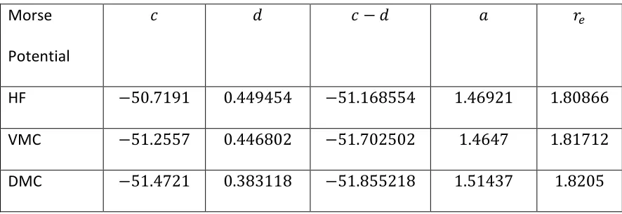
Table 3 Morse curve data for 𝐓𝐡𝐎. ... 67
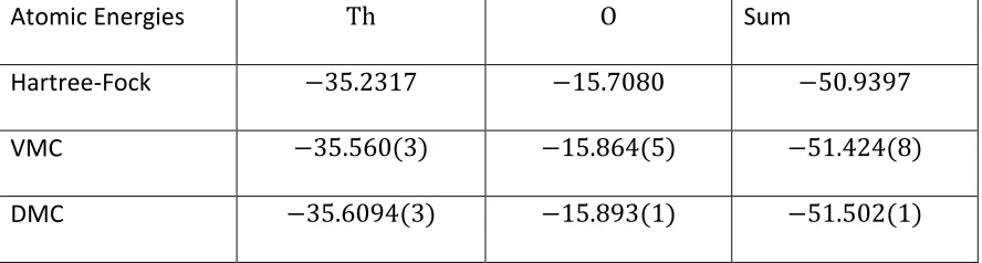
Table 4 Atomic energies for 𝐓𝐡𝐎. ... 68
Table 5 Dielectric Constant of 𝐓𝐡𝐎𝟐 along [100] direction. ... 81
Table 6 Enthalpies of formation for 𝐓𝐡𝐎𝟐 ... 88
Table 7 Fixed-node error for 𝐍𝐞 atom... 108
Table 8 Fixed-node error for 𝐍 and 𝐏 atom. ... 108
vii
LIST OF FIGURES
Figure 1 HEG Hartree-Fock Exchange Function 𝐹(𝑥) ... 26
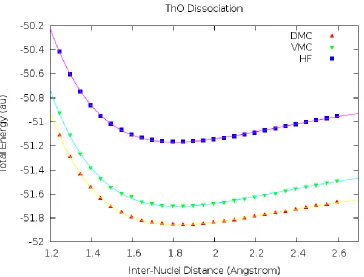
Figure 2 𝐓𝐡𝐎 Dissociation Curve ... 65
Figure 3 𝐓𝐡𝐎 DMC dissociation curve ... 67
Figure 4 Dipole Moment of ThO. ... 69
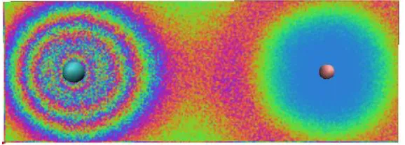
Figure 5 two-body energy density for ThO molecule. ... 70
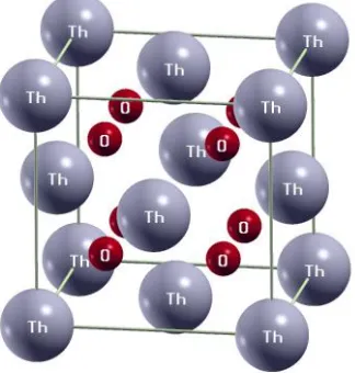
Figure 6 Crystal structure of 𝐓𝐡𝐎𝟐. Fluorite phase (𝐹𝑚3̅𝑚) at normal pressure. ... 72
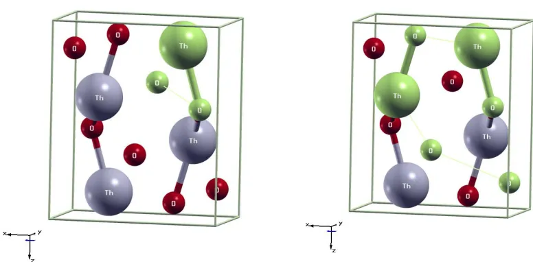
Figure 7 Crystal structure of 𝐓𝐡𝐎𝟐. Cotunnite phase (𝑃𝑛𝑚𝑎) at high pressure. ... 73
Figure 8 Total and partial (atomic symmetry projected) DOS. ... 74
Figure 9 Electron Charge distribution on [110] plane of fluorite thoria. ... 75
Figure 10 Band structure of 𝐹𝑚3̅𝑚 phase 𝐓𝐡𝐎𝟐 calculated using PBE functional. ... 76
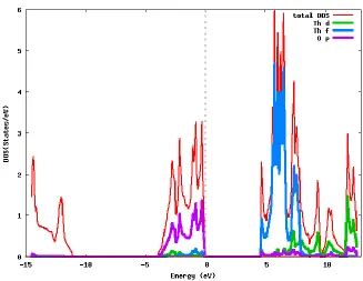
Figure 11 DOS for 𝐹𝑚3̅𝑚 phase 𝐓𝐡𝐎𝟐from PBE calculation. ... 78
Figure 12 Applied and Response Electric Field on 𝐓𝐡𝐎𝟐. ... 80
Figure 13 Electron density 2d map sliced through 3 inequivalent atoms in 𝑃𝑛𝑚𝑎 phase primitive cell... 83
Figure 14 Electron density 2d map in a 4-atom plane in 𝑃𝑛𝑚𝑎 phase primitive cell. ... 83
Figure 15 DFT Cohesive Energy per formula unit (𝐓𝐡𝐎𝟐) in Rydberg. ... 84
Figure 16 Static structure factor for 𝐓𝐡𝐎𝟐. ... 86
Figure 17 Infinite cell size extrapolation ... 87
Figure 18 DMC Cohesive Energy per formula unit (𝐓𝐡𝐎𝟐) in Rydberg. ... 89
Figure 19 [𝟒𝑺(𝟏𝒔𝟐𝒔𝟑𝒔)] HF nodes... 104
Figure 20 Relative positions of electrons. ... 105
Figure 21 Nodal domains have been reduced to two after the introduction of angular correlation. ... 105
1
Chapter 1 Introduction to Electronic Structure Calculation
Electrons and nuclei are the fundamental particles that determine the nature of the matter
of our everyday world: atoms, molecules, condensed matter, artificial and biological
material. Even life itself can be viewed as an “emergent” behavior and a “meta-stable” state
of these fundamental particles.
Understanding of the behavior of electrons holds the key to understanding material
properties and development and application of new materials. However, correctly
describing their behavior needs the language of quantum mechanics.
Fundamental ideas of quantum mechanics were formulated and developed in the first half
of the 20th century. The theory, unintuitive to many, has demonstrated a surprising accuracy
and predictive power.
With the help of quantum mechanics, we can see how electrons form the “quantum glue”
that holds together nuclei in molecules and materials and how their quantum states
determine the vast array of electrical, optical, magnetic and behavioral properties of
materials.
One of the most basic and key mathematical tools in quantum mechanics is non-relativistic
Schrodinger’s Equation, whose solutions, i. e. many-body wave functions, are explicit
2
or even approximating these solutions correctly for various circumstances1 ranks among the
greatest challenges of theoretical physics.
Some of the standard approaches to the solution will be briefly described in following
chapters.
1 Sometimes in order get the approximate solution, people modified Schrodinger’s equation or
3 Non-relativistic Schrodinger equation
The form of the Schrödinger equation depends on the physical situation. The most general
form is:
Time-dependent Schrödinger equation
𝑖ℏ 𝜕
𝜕𝑡Ψ = 𝐻̂ Ψ
This equation describes the evolution of many-body quantum state Ψ for system with
Hamiltonian Ĥ.
If Ψ(R) is an eigenstate of Ĥ with eigenvalue E, where R are spatial coordinates of
particles, then solution Ψ(R)e−iEℏt satisfies the equation. The time-dependent piece could
be separated out as a simple “oscillating” factor. Since any quantum state could be seen as
a linear superposition of energy eigenstates, the dynamics of the system could be known in
theory if we have all the eigenstates available. To find Ĥ eigenstates, we have:
Stationary Schrodinger equation
𝐸 Ψ = 𝐻̂ Ψ
However, finding all the eigenstates has been proven to be difficult except for simplest
cases (like non-interacting Hamiltonians). People could argue that in most cases, it is near
impossible to know exactly and check all the solutions.
For a generic interacting Hamiltonian, total energy grows linearly with system size while
number of states/solutions Ψ grows exponentially. This means average energy spacing
4
resolve these energy differences becomes exponentially large. For a 200 electron system,
range of total energy for all eigenstates is about the magnitude of 200 eV, while the total
number of eigenstates is, say, about 2200; the average energy difference between two
states 200eV2200 ≈ 10−58eV ; the time needed to resolve this difference ≈ ℏ 200eV/2200≈
5.288529 × 1042 seconds ≈ 1.2 × 1025 × universe age (~ 14 Gyr ) . This means even if
we could find all the solutions, it would be impossible to check all of them in experiments.
Therefore, for solutions of explicit many-body wave function, we want to focus on the
ground state and low-lying excitations first which provide the easiest access and sometimes
most valuable and interesting information on quantum phenomenon.2
Another important observation is that quite often the wave function in chemical
environment Ψ(𝑅𝑒, 𝑅𝑛), 𝑅𝑒 being coordinates of electrons, 𝑅𝑛 being coordinates of
nuclei/ions3, can be separated into a product of electronic and nuclear wave function, since
2 For an ensemble of excited states, techniques that don’t involve explicit many-body wave functions
are preferred, for example, Path Integral Monte Carlo.
3 To avoid confusion with concepts in nuclear physics, we sometimes call nuclei ions as they are bare
5
nuclei are much heavier than electrons (details will be discussed in the next section). This
enables us to focus on the electronic part and nuclear part separately. This separation is
called Born-Oppenheimer approximation.
Born-Oppenheimer Approximation
If we write Ψ(𝑅𝑒, 𝑅𝑛) = Ψe(𝑅𝑒, 𝑅𝑛) Ψn(𝑅𝑛), and ignore kinetic energy operator of ions
on Ψ𝑒, the Schrodinger equation can be broken apart:
𝐻̂ Ψ = ( 𝐻̂𝑒+ 𝑇̂𝑛) Ψ = (𝐻̂𝑒Ψ𝑒+ Ψ𝑒𝑇̂𝑛) Ψ𝑛 = Ψ𝑒[𝑇̂𝑛+ 𝐸𝑒(𝑅𝑛)]Ψ𝑛(𝑅𝑛)
, where 𝑇̂𝑛 is kinetic energy operator for nuclei, 𝐻̂𝑒 contains all the rest like kinetic energy
for electrons, ion-electron potential energy, ion-ion potential energy and electron-electron
interaction, Ψ𝑒 is an eigenvector of 𝐻̂𝑒 with eigenvalue 𝐸𝑒.
Thus we end up with two equations to solve, one for electrons and one for nuclei, 𝑅𝑛 are
fixed in the former and 𝑅𝑒 don’t appear in the latter:
𝐻̂𝑒(𝑅𝑛)Ψ𝑒 = 𝐸𝑒(𝑅𝑛) Ψ𝑒
[ 𝑇̂𝑛+ 𝐸(𝑅𝑛) ] Ψn= 𝐸 Ψn
Notice the dependence of 𝐻̂𝑒 on 𝑅𝑛 through ion-electron potential and ion-ion potential,
naturally implies the dependence of eigenvalue 𝐸𝑒 on 𝑅𝑛. In practice, one might vary these
positions𝑅𝑛 in small steps and repeatedly solving the electronic Schrödinger equation to
6
𝐸𝑒(𝑅𝑛) , with all the information about electrons in the system, enters the nuclear
equation as an potential energy for nuclei and is commonly referred to as PES(Potential
Energy Surface) from nuclei’s point of view4. Now one can proceed to solve for the motion
of nuclei, which for small molecules often involves translation and several vibrational and
rotational modes.
It can be shown that Born-Oppenheimer approximation is valid whenever PESs, obtained
from solutions of electronic Schrodinger equation 𝐻̂𝑒 Ψ𝑒𝑘 = 𝐸𝑒𝑘 Ψ𝑒𝑘 are well separated:
𝐸𝑒0(𝑅
𝑛) ≪ 𝐸𝑒1(𝑅𝑛) ≪ 𝐸𝑒2(𝑅𝑛) ≪ ⋯ ∀ 𝑅𝑛
In order to show this, first we recognize that true solution to the original equation can
always be expanded in terms of Ψ𝑒𝑘 :
Ψ = ∑ Ψ𝑛𝑘(𝑅
𝑛) Ψ𝑒𝑘(𝑅𝑒, 𝑅𝑛) k
Also in the basis of Ψ𝑒𝑘, it is easy to see 𝐻̂ would take on matrix form
𝐻𝑘𝑘′ = 𝐸𝑒𝑘 𝛿𝑘𝑘′ + 𝑇̂𝑘𝑘′, 𝑤ℎ𝑒𝑟𝑒 𝑇̂𝑘𝑘′ = 〈 Ψ𝑒𝑘| 𝑇̂𝑛| Ψ𝑒𝑘′〉
4 Because this procedure of recomputing the electronic wave functions as a function of an
infinitesimally changing geometry of ions is reminiscent of the conditions for the adiabatic
theorem, this manner of obtaining a PES is often referred to as the adiabatic
7
𝑅𝑛 appears in all terms so it is omitted here and in the following derivation; expectation 〈〉 is
understood to be taken over 𝑅𝑒.
Notice that 𝑇̂𝑘𝑘′ is an operator that can still act on Ψ𝑛𝑘′ , as
𝑇̂𝑛 = ∑ 𝑷𝐼2 2𝑀𝐼 𝑖
𝐼 ∈ 𝑛𝑢𝑐𝑙𝑒𝑖
𝑇̂𝑘𝑘′ = 〈Ψ𝑒𝑘| Ψ𝑒𝑘′〉 𝑇̂𝑛+ ∑ 1 𝑀𝐼 𝐼 〈Ψ𝑒𝑘| 𝑷 𝐼 |Ψ𝑒𝑘 ′ 〉 ∙ 𝑷𝐼+ 〈 Ψ𝑒𝑘|( 𝑇̂ 𝑛| Ψ𝑒𝑘 ′ 〉 )
= 𝛿𝑘𝑘′ 𝑇̂𝑛 + ∑ 1 𝑀𝐼 𝐼
〈Ψ𝑒𝑘| 𝑷𝐼 |Ψ𝑒𝑘′〉 ∙ 𝑷𝐼 + 〈 Ψ𝑒𝑘|( 𝑇̂𝑛| Ψ𝑒𝑘′〉 )
Now we see Born-Oppenheimer approximation is essentially only keeping the first term
here and ignoring the last two, which is valid when they are small.
First we know that when 𝑘 = 𝑘′ 〈Ψ𝑒𝑘|𝑷𝐼|Ψ𝑒𝑘〉 = 0 if we assume non-degeneracy of Ψ𝑒𝑘 and
time-reversal symmetry of our Hamiltonian; this could easily be shown by the properties of
time-reversion operator directly or by showing that Ψ𝑒𝑘 can be expressed as real wave
function in this case, so that 〈Ψ𝑒𝑘|𝑷𝐼|Ψ𝑒𝑘〉 = (𝑠𝑜𝑚𝑒 𝑐𝑜𝑛𝑠𝑡𝑎𝑛𝑡) × ∇𝒓𝐼〈Ψ𝑒𝑘|Ψ𝑒𝑘〉 = 0, as
normalization is a constant.
When 𝑘 ≠ 𝑘′
〈Ψ𝑒𝑘| 𝑷𝐼 | Ψ𝑒𝑘′〉 = 〈Ψ𝑒𝑘|[𝑷𝐼 , 𝐻̂𝑒]|Ψ𝑒𝑘′〉 𝐸𝑒𝑘′ − 𝐸𝑒𝑘 The numerator 〈Ψ𝑒𝑘|[𝑷𝐼 , 𝐻̂𝑒]|Ψ𝑒𝑘′〉 = −𝑖ℏ ∑ 𝑍𝐼 𝑗 〈Ψ𝑒𝑘| 𝒓𝐼𝑗
𝑟𝐼𝑗3 | Ψek ′
8
is proportional to the Coulomb force on nucleus 𝐼 from joint electronic distribution 𝜌𝑒
shown below.
𝑭𝐼 = −𝑍𝐼∫ 𝜌𝑒(𝒓′)
|𝒓𝐼− 𝒓′|3 (𝒓𝐼− 𝒓
′) 𝑑𝒓′
𝜌𝑒(𝒓′) = 〈Ψ𝑒𝑘|𝜌̂(𝒓′)|Ψ𝑒𝑘 ′
〉
= ∑ ∫ δ(𝒓𝑗− 𝒓′)Ψ𝑒𝑘∗(𝑅𝑛 , 𝒓1, 𝒓2, … , 𝒓𝑛) ∙ Ψ𝑒𝑘′(𝑅𝑛, 𝒓1, 𝒓2, … , 𝒓𝑛) ∏ 𝑑𝒓𝑠 𝑠 𝑗
Dot product between Ψ𝑒𝑘 and Ψ𝑒𝑘′ would sum over possible spin dimensions.
Notice ∫ 𝜌𝑒(𝒓′) 𝑑𝒓′= 0 due to orthogonality of Ψ𝑒𝑘 and Ψ𝑒𝑘′.
One can also notice that if both Ψ𝑒𝑘 and Ψ𝑒𝑘′ are expressed as a linear combination of
determinants of single-particle orbitals, then only pairs of determinants, one from each
wave function, that are different by at most one single-particle orbital would survive as the
density operator in 𝜌𝑒 is an one-particle operator and can be rewritten using a single pair of
creation and annihilation operators.
𝜌𝑒(𝒓) = ∑〈Ψ𝑒𝑘|𝜓𝜎+(𝒓)𝜓𝜎(𝒓)|Ψ𝑒𝑘 ′
〉 𝜎
= ∑ 〈Ψek|𝑐 𝑖,𝜎+ 𝑐𝑗,𝜎| 𝑖,𝑗,𝜎 Ψ𝑒𝑘′〉 𝜙 𝑖,𝜎 ∗ (𝒓)𝜙 𝑗,𝜎(𝒓)
, where 𝜙𝑖,𝜎(𝑖 ∈ 𝑖𝑛𝑡𝑒𝑔𝑒𝑟𝑠, 𝜎 ∈ 𝑠𝑝𝑖𝑛 𝑙𝑎𝑏𝑒𝑙𝑠) are single-particle orbitals.
9 𝑇̂𝑘𝑘′ = 𝛿𝑘𝑘′ 𝑇̂𝑛 + (1 − 𝛿𝑘𝑘′) ∑𝑖ℏ
𝑀𝐼 𝐼 𝑭𝐼,𝑘𝑘′ 𝐸𝑒𝑘′ − 𝐸𝑒𝑘∙ 𝑷𝐼+ ∑ (𝑖ℏ)2 2𝑀𝐼 𝐼, 𝑘′′≠𝑘 𝑜𝑟 𝑘′ 𝑭𝐼,𝑘𝑘′′ 𝐸𝑒𝑘′′ − 𝐸𝑒𝑘 ∙ 𝑭𝐼,𝑘′′𝑘′ 𝐸𝑒𝑘′ − 𝐸𝑒𝑘′′
If we define Hermitian operator 𝑷𝐼,𝑒 (off-diagonal impetus on nucleus 𝐼) by its matrix
elements in Ψ𝑒𝑘 basis as
(𝑷𝐼,𝑒)𝑘𝑘′ = {𝑖ℏ
𝑭𝐼,𝑘𝑘′ 𝐸𝑒𝑘′ − 𝐸𝑒𝑘
, 𝑘 ≠ 𝑘′
0, 𝑘 = 𝑘′
, we can write
𝑇̂𝑛 = ∑
(𝑷𝐼,𝑛+ 𝑷𝐼,𝑒)2 2𝑀𝐼 𝐼
Operator 𝑷𝐼,𝑛, same as 𝑷𝐼 in 𝑇̂𝑘𝑘′, would not act on electronic wave function as all that has
been absorbed into 𝑷𝐼,𝑒. We see 𝑷𝐼,𝑒 and 𝑷𝐼,𝑛 are in effect nothing but 𝑷𝐼in the Hilbert
space of electron wave function and ion wave function respectively.
Since all |𝑭𝑖| are finite, we see that, if |𝐸𝑒𝑘′
− 𝐸𝑒𝑘| ≫ 1 ∀ 𝑘 ≠ 𝑘′, the last two terms in 𝑇̂ 𝑘𝑘′
expression can be duly dropped, or equivalently speaking, 𝑷𝐼,𝑒’s contribution to 𝑇̂𝑛 can be
neglected.
However, PESs could be very close to or sometimes even crossing each other at some 𝑅𝑛. In
these cases, we are forced to consider the coupling of different electronic eigenstates due
10
diagonalize 𝐻̂𝑘𝑘′ properly in dimensions no less than the number of PESs close to each
other.
One situation of particular interest and importance is when 𝑅𝑛 are at equilibrium positions
in a crystal environment. Then displacements of lattice sites from 𝑅𝑛, if assumed to be
small, will only increase 𝐸(𝑅𝑛) in the second order of 𝛿𝑅𝑛. In this case, it is well known
that the lattice oscillations can be decomposed into normal modes that can be
characterized by phonons, i.e., Hamiltonian 𝑇̂𝑛+ 𝐸(𝑅𝑛) is equivalent to 2𝑀1
𝐼(∑ 𝑃𝒌 +𝑃
𝒌+ 𝒌
𝑀𝐼2𝜔2(𝒌)𝑄𝒌+𝑄𝒌), where 𝑃𝒌 =√𝑁1 ∑ 𝑃𝐼 𝐼𝑒−𝑖𝒌∙𝒓𝐼 , 𝑄𝒌=√𝑁1 ∑ 𝛿𝑟𝐼 𝐼𝑒−𝑖𝒌∙𝒓𝐼, 𝒌 lies in the first
Brillouin Zone and 𝑁 is the total number of ions (We have assumed that there’s a single kind
of ions here with mass 𝑀𝐼, which can be easily generalized to multiple ones with a proper
choice of basis. We have also suppressed the label for polarization. You can think that we
only focus on longitudinal modes of vibrations here as an example).
In this case, ignoring coupling/off-diagonal terms for kinetic energy operator, motions of
ions are well known to be phonons with frequencies 𝜔𝒌, 𝒌being the wavevector. Starting
with these electronic states (ones we solved from periodic potential provided by fixed ions)
and phonon states, we can calculate the effect of their coupling as perturbation if their
effect is assumed to be small albeit non-zero. Another way to look at the problem from
time-dependent perturbation point of view is that if there are transitions between
11
Hamiltonian, the adiabatic approximation which lies at the heart of Born-Oppenheimer
approximation breaks down.
However, in practical calculation of electron-phonon coupling, people always start with a
simpler and also more intuitive Hamiltonian (Bloch 1928):
∑ 𝛿𝒓𝐼∙ ∇𝒓𝐼𝑈𝑛(𝒓𝑗− 𝒓𝐼) 𝐼∈𝑖𝑜𝑛𝑠,𝑗∈𝑒𝑙𝑒𝑐𝑡𝑟𝑜𝑛𝑠
, 𝑈𝑛 stands for ion-electron potential energy here being Coulomb potential; 𝛿𝒓𝐼 acts on the
wavefunction of ions while the rest acts on the electronic wavefunction. We’ll refer to this
form as Bloch potential.
This looks different from our coupling term, and we usually think this change in ion-electron
potential energy should have been included in PES thus well captured in Born-Oppenheimer
approximation. But the truth is that this coincides with PES only to the first order of 𝛿𝒓𝐼 and
the counter-intuitive bit is that this generates the same first order electron-phonon
scattering probability as the second term in our 𝑇̂𝑘,𝑘′ expression:
The matrix representation (in electronic eigenstates 𝑛, 𝑚; we switched 𝑘, 𝑘′ to 𝑛, 𝑚 to avoid
confusion with wavevector 𝒌) of the Bloch potential is
∑ −𝑖𝑘 1 √𝑁𝑄𝒌𝑒
𝑖𝒌∙𝒓𝐼 1 √𝑁 𝑈𝒌′𝑒
−𝑖𝒌′∙𝒓𝐼∫ 𝑑𝒓 𝑒𝑖𝒌′∙𝒓〈𝑛|𝜌̂(𝒓)|𝑚〉
𝒌,𝒌′,𝑰
= −𝑖 ∑ 𝑘√ ℏ
2𝑀𝐼𝜔𝒌 (𝑎𝒌+ 𝑎−𝒌 + ) 𝑈
12
, where 𝜌̂𝒌+ = ∫ 𝑑𝒓 𝑒𝑖𝒌∙𝒓 𝜌̂(𝒓), would transfer electron to a state with additional
momentum 𝒌, which is obvious in plane wave representation, as 𝜌̂(𝒓) =
1
𝑉∑ 𝑐𝒑′ +(𝒓)𝑐
𝒑(𝒓)
𝒑,𝒑′ 𝑒𝑖(𝒑−𝒑′)∙𝒓 shows 𝜌̂𝒌+ = ∑ 𝑐𝒑 𝒑+𝒌+ 𝑐𝒑. Notice that conservation of total
momentum of electrons and phonons (up to a reciprocal lattice vector of course as |𝑛〉
and |𝑚〉 are many-body Bloch states) is apparent here.
Similarly, we can express our coupling term
∑𝑖ℏ 𝑀𝐼 𝐼 𝑭𝐼,𝑛𝑚 𝐸𝑒𝑚− 𝐸𝑒𝑛∙ 𝑷𝐼 = ∑ −𝑖ℏ 𝑀𝐼(𝐸𝑒𝑚− 𝐸𝑒𝑛) 𝐼 𝑷𝐼∙ ∫ 𝑑𝒓 ∇𝒓𝐼𝑈𝑛(𝒓 − 𝒓𝐼)〈𝑛|𝜌̂(𝒓)|𝑚〉 = − 𝑖ℏ 𝑀𝐼(𝐸𝑒𝑚− 𝐸𝑒𝑛)∑ 𝑃𝒌 + 𝒌 (−𝑖𝑘)𝑈𝒌〈𝑛|𝜌̂𝒌+|𝑚〉 = − 𝑖ℏ 𝑀𝐼(𝐸𝑒𝑚− 𝐸𝑒𝑛)∑(−𝑖)√ ℏ𝑀𝐼𝜔𝒌
2 (𝑎𝒌− 𝑎−𝒌+ ) 𝒌
(−𝑖𝑘)𝑈𝒌〈𝑛|𝜌̂𝒌+|𝑚〉
= −𝑖 ∑ 𝑘√ ℏ
2𝑀𝐼𝜔𝒌 𝒌 (𝑎𝒌 ℏ𝜔𝒌 𝐸𝑒𝑛− 𝐸 𝑒𝑚+ 𝑎−𝒌 + ℏ𝜔𝒌 𝐸𝑒𝑚− 𝐸 𝑒𝑛) 𝑈𝒌〈𝑛|𝜌̂𝒌 +|𝑚〉
Notice that this is exactly the same as Bloch potential if energy conservation is satisfied, i.e.,
when a phonon of energy ℏ𝜔𝒌 gets destroyed, electronic states must gain the same amount
of energy (𝐸𝑒𝑛− 𝐸𝑒𝑚 = ℏ𝜔𝒌) and similarly for the creation of a phonon.
To the first order of perturbation, the only non-zero contribution to coupling is coming
13
and 𝑷𝐼 are destroying or creating different states. Degeneracy in total energy of the system
means the total energy of electron and phonon states must be conserved. Therefore, the
second term in our 𝑇̂𝑛 expression has the same effect as electron-phonon coupling of Bloch
potential to the first order. The last term in our 𝑇̂𝑛 expression, 𝑷𝐼,𝑒 2
2𝑀𝐼 is not only small but
often has very weak to little dependence on 𝒓𝐼, so can be safely ignored(J.M.Ziman, 1960).
Electron-phonon coupling has many consequences. Probably the most familiar one is the
scattering of electrons by phonons, which is an important cause of resistance in metals. A
second consequence is the absorption of phonons by the electrons, which offers a
mechanism for the attenuation of a sound wave, or, in higher order, for thermal resistance
in metals. Two other closely related renormalization effect, typical manifest of interactions,
are the dressing of electron as a quasiparticle (called polaron) due to interaction with
phonon cloud, which is responsible for the colossal magneto-resistance effect in manganite,
and vice versa as electron gas could be polarized by motion of ions, which in turn changes
the effective interaction among ions and hence changes the characteristic phonon
frequency.
We’ll not go into the application of electron-phonon coupling here. But we should always
caution ourselves whether it is safe to neglect it. We see that one sufficient, but maybe not
necessary, condition is that energy spacing between electronic eigenstates are way larger
than possible phonon energy ℏ𝜔𝒌, whose average value is around 𝑘𝑇. So in general this
14
which exists, as its name implies, at zero temperature. One clear exception to this condition
is metal at room temperature, as it is zero gap material.
In the following pages of this chapter, we’ll assume Born-Oppenheimer approximation is
valid and focus on the electronic equation with 𝑅𝑛 fixed, or more generally, a
non-relativistic Schrodinger equation with Hamiltonian for identical particles in the form:
𝐻 = ∑ (𝑝𝑖 2
2𝑚+ 𝑣𝑒𝑥𝑡(𝒓𝑖)) 𝑖
+ ∑ 𝑣(𝒓𝑖𝑗) 𝑖<𝑗
We’ll drop hat notation on operators as they should be clear from context.
Symbol 𝑣 denotes interaction among particles while 𝑣𝑒𝑥𝑡 is the external potential felt by
15
Chapter 2 Hartree-Fock Method
We know how to solve the Schrodinger equation if Hamiltonian is non-interacting,
i.e. one that only contains one-body terms:
𝐻0 = ∑ (𝑝𝑖 2
2𝑚+ 𝑣𝑒𝑥𝑡(𝒓𝑖)) 𝑖
In this approximation the eigenstates of 𝐻0 may be written as the product of singe-particle
wave functions, each of which satisfies the equation (ℏ = 1)
(− ∇ 2
2𝑚+ 𝑣𝑒𝑥𝑡(𝒓)) 𝜙𝑘(𝒓) = 𝜀𝑘𝜙𝑘(𝒓)
If we can approximate electron-electron interaction by some effective 𝑣𝑒𝑥𝑡(𝒓), then the
problem reduces to an independent-particle one. However, the proper choice of 𝑣𝑒𝑥𝑡 to
best represent the effects of electron-electron interaction is a subtle problem. Or
theoretically speaking, it is downright impossible because the very fact that
independent-particle solutions are products of single-independent-particle wave functions means behaviors of
particles are not correlated as they should. However, it is valid to ask how we can do this in
a way that is least unreasonable. In this thesis, we’ll call using products of a set of
single-particle orbitals to describe many-body states independent particle approximation. We’ll illustrate the idea using electrons, which are also the main focus of current thesis, as
16
To begin with, 𝑣𝑒𝑥𝑡 should incorporate, at least approximately, the fact that electrons feel
the electric fields of all other electrons. If we treat the remaining electrons as a smooth
distribution of charge with charge density 𝜌, the potential energy of given electron in their
field would be
𝑉(𝒓) = ∫ 𝑑𝒓′ 𝜌(𝒓′) |𝒓 − 𝒓′|
Furthermore, if we insisted on an independent electron picture, ground state 𝜌 can be
easily expressed as
𝜌(𝒓) = ∑〈𝜓𝜎+(𝒓)𝜓 𝜎(𝒓)〉 𝜎 = ∑〈𝑐𝑖,𝜎+ 𝑐 𝑗,𝜎〉 𝜙𝑖,𝜎∗ (𝒓) 𝑖,𝑗,𝜎 𝜙𝑗,𝜎(𝒓) = ∑〈𝑛𝑖,𝜎〉|𝜙𝑖,𝜎(𝒓)| 2 𝑖,𝜎
, where 𝑛𝑖,𝜎 are number operators and 〈𝑛𝑖,𝜎〉 are current occupation numbers (1 for
occupied and 0 for unoccupied).
By adding this 𝑉(𝒓) to 𝑣𝑒𝑥𝑡 that originally only contains contribution from ions, we arrive at
a set of self-consistent equations:
[ − ∇2
2𝑚+ 𝑉𝑖𝑜𝑛(𝒓)] 𝜙𝑖,𝜎(𝒓) + [∑ ∫ 𝑑𝒓′ 〈𝑛𝑖,𝜎′〉
|𝜙𝑗,𝜎′(𝒓′)|2 |𝒓 − 𝒓′| 𝑗,𝜎′
] 𝜙𝑖,𝜎(𝒓) = 𝜀𝑖,𝜎𝜙𝑖,𝜎(𝒓)
This set of equations is known as Hartree equations. We call these non-linear equations self-consistent as the problem (Hamiltonian) is dependent on the solution (𝜙𝑖𝑠) so that its
solution has to be self-consistent. And in practice, it is often solved by iteration. Since the
potential/field is generated from solutions of previous iteration, this kind of methods are
17
differences between two solutions of adjacent iterations is smaller than certain preset
threshold that deemed accurate enough for the situation.
The Hartree equations have a fundamental inadequacy that might not evident from the
simple derivation above. The defect emerges if we return to the original Hamiltonian and
cast it into the equivalent variational form. It becomes apparent when we can compare the
expectation of interaction in original Hamiltonian and our Hartree approximation.
Electron-electron interaction in second quantized form:
1
2∑ ∫ 𝑑𝒓𝑑𝒓′𝜓𝜎+(𝒓)𝜓𝜎+′(𝒓′) 1
|𝒓 − 𝒓′|𝜓𝜎′(𝒓′)𝜓𝜎(𝒓) 𝜎,𝜎′
Electron-electron interaction in Hartree approximation:
1
2∑ ∫ 𝑑𝒓𝑑𝒓′〈𝜓𝜎+(𝒓)𝜓𝜎(𝒓)〉 1
|𝒓 − 𝒓′| 〈𝜓𝜎+′(𝒓′)𝜓𝜎′(𝒓′)〉 𝜎,𝜎′
Even with the assumption of independent particle approximation (that our many-body state
is a simple product of single-particle states |Ψ〉 = ∏i,σi𝑐𝑖,𝜎+𝑖|0〉, 𝑐𝑖,𝜎𝑖
+ being the corresponding
creation operator for spin orbital 𝜙𝑖,𝜎; we don’t construct spin eigenstates here), the
expectation of true Coulomb interaction is not just what we have in Hartree approximation,
which can be clearly seen from two-body density matrix:
𝜌2(𝒓, 𝒓′) = ∑〈Ψ|𝜓
𝜎+(𝒓)𝜓𝜎+′(𝒓′)𝜓𝜎′(𝒓′)𝜓𝜎(𝒓)|Ψ〉 𝜎,𝜎′
18 = ∑〈𝜓𝜎+(𝒓)𝜓𝜎(𝒓)〉〈𝜓+𝜎′(𝒓′)𝜓𝜎′(𝒓′)〉 𝜎,𝜎′ − ∑〈𝜓𝜎+(𝒓)𝜓𝜎(𝒓′)〉〈𝜓𝜎+(𝒓′)𝜓𝜎(𝒓)〉 𝜎 = 𝜌(𝒓)𝜌(𝒓′) − ∑|𝜌
𝜎(𝒓, 𝒓′)|2 𝜎
Expectation is understood to be taken over |Ψ〉. The first step is from the observation that,
when sandwiched between |0〉, two sets of 𝜓 and 𝜓+ have to pair with two
orbitals 𝑐𝑖,𝜎+ 𝑖, 𝑐
𝑖,𝜎𝑖, 𝑐𝑗,𝜎𝑗 + , 𝑐
𝑗,𝜎𝑗 in Ψ. If there is an even number of crossings among these four
pairings we could find it in the first term of the 2nd line, while others (odd number of
crossing gives an extra negative sign) could be found it in the second term of the 2nd line.
Notice that possible situation for 𝑖 = 𝑗 𝑎𝑛𝑑 𝜎𝑖 = 𝜎𝑗 the same contribution will be made to
the two terms in subtraction so that we recover the original expression. We see that even
with independent particle approximation, two-body density is not a simple product of two
one-body densities when two interacting electrons share the same spin(𝜎 = 𝜎′). The first
term which is a product of two densities leads to the energy term we have in Hartree
approximation. This energy called Hartree energy. The second term, associated with
off-diagonal one-body density matrix, when integrated with Coulomb potential over space
gives so called exchange energy. More explicitly, 𝑈𝐻𝑎𝑟𝑡𝑟𝑒𝑒 =1
2 ∫ 𝑑𝒓𝑑𝒓′
𝜌(𝒓)𝜌(𝒓′) |𝒓 − 𝒓′|
𝑈𝑒𝑥𝑐ℎ𝑎𝑛𝑔𝑒= − 1
2∫ 𝑑𝒓𝑑𝒓′∑
|𝜌𝜎(𝒓, 𝒓′)|𝟐 |𝒓 − 𝒓′| 𝜎
19 𝜌𝜎(𝒓, 𝒓′) = 〈𝜓𝜎+(𝒓′)𝜓𝜎(𝒓)〉 = ∑〈𝑐𝑖,𝜎+ 𝑐𝑗,𝜎〉 𝜙𝑖,𝜎∗ (𝒓′) 𝑖,𝑗,𝜎 𝜙𝑗,𝜎(𝒓) = ∑〈𝑛𝑖,𝜎〉 𝑖,𝜎 𝜙𝑖,𝜎(𝒓)𝜙𝑖,𝜎∗ (𝒓′)
Therefore, the exact variational evaluation of electron-electron interaction for our Ψ
contains not only 𝑈𝐻𝑎𝑟𝑡𝑟𝑒𝑒 but also 𝑈𝑒𝑥𝑐ℎ𝑎𝑛𝑔𝑒. Thus to find the best Ψ within independent
particle approximation, i.e. the set of occupied orbitals, we only have to minimize total
energy with both 𝑈𝐻𝑎𝑟𝑡𝑟𝑟𝑒 and 𝑈𝑒𝑥𝑐ℎ𝑎𝑛𝑔𝑒 included. With the help of derivatives
𝛿𝑈𝐻𝑎𝑟𝑡𝑟𝑒𝑒
𝛿𝜙𝑖,𝜎∗ (𝒓) = ∫ 𝑑𝒓′
𝜌(𝒓′)
|𝒓 − 𝒓′| 𝜙𝑖,𝜎(𝒓) = ∑ ∫ 𝑑𝒓′ 〈𝑛𝑗,𝜎′〉
|𝜙𝑗,𝜎′(𝒓′)|2 |𝒓 − 𝒓′| 𝑗,𝜎′ 𝜙𝑖,𝜎(𝒓) 𝛿𝑈𝑒𝑥𝑐ℎ𝑎𝑛𝑔𝑒 𝛿𝜙𝑖,𝜎∗ (𝒓) = − ∫ 𝑑𝒓′ 𝜌𝜎(𝒓′, 𝒓) |𝒓 − 𝒓′| 𝜙𝑖,𝜎(𝒓′) = − ∑ ∫ 𝑑𝒓′ 〈𝑛𝑗,𝜎〉 𝜙𝑗,𝜎(𝒓)𝜙𝑗,𝜎∗ (𝒓′) |𝒓 − 𝒓′| 𝑗 𝜙𝑖,𝜎(𝒓′)
, we can minimize 〈Ψ|𝐻|Ψ〉 with constrains ∫ 𝑑𝒓 𝜙𝑖,𝜎∗ (𝒓)𝜙𝑖,𝜎(𝒓) = 1 ∀ 𝑖, σ.
We arrive at a set of equations for 𝜙𝑖
[− 𝛻2
2𝑚+ 𝑉𝑖𝑜𝑛(𝑟)] 𝜙𝑖,𝜎(𝒓) + [∑ ∫ 𝑑𝒓′ 〈𝑛𝑗,𝜎′〉
|𝜙𝑗,𝜎′(𝒓′)|2 |𝒓 − 𝒓′| 𝑗,𝜎′ ] 𝜙𝑖,𝜎(𝒓) − ∑ ∫ 𝑑𝒓′〈𝑛 𝑗,𝜎〉 𝜙𝑗,𝜎∗ (𝒓′)𝜙 𝑖,𝜎(𝒓′) |𝒓 − 𝒓′| 𝑗 𝜙𝑗,𝜎(𝒓) = 𝜀𝑖,𝜎𝜙𝑖,𝜎(𝒓)
Eigenvalue𝑠 𝜀𝑖 are Lagrange multipliers during minimization and they resemble
single-particle energies. Their physical meaning will be clarified shortly afterwards.
Notice that the exchange term can be simply obtained from the Hartree term (when σ = σ′)
by exchanging 𝑖 and 𝑗 for 𝜙𝑗,𝜎(𝒓′)𝜙
𝑖,𝜎(𝒓). This set of SCF equations is called Hartree-Fock equations. The operator we defined here is called Fock operator, which is our new effective
20
We can drop all the spin labels if we don’t distinguish between orbitals [and their
eigenvalues] of different spin, just be careful that once we dropped the spin label the
occupation number in Hartree term would be 2 for doubly occupied orbitals while exchange
term is always counting occupation with the same spin. This is called Restricted
Hartree-Fock. The method in which we accommodate different orbitals for different spins is named
Unrestricted Hartree-Fock.
Total energy of Hatree-Fock method could be calculated after the iterations converged. If
we simply added up 𝜀𝑖,𝜎, we would have counted electron-electron interaction twice.
Therefore,
𝐸𝑡𝑜𝑡𝑎𝑙 = ∑〈𝑛𝑖,𝜎〉 𝜀𝑖,𝜎 𝑖,𝜎
− 𝑈𝐻𝑎𝑟𝑡𝑟𝑒𝑒− 𝑈𝑒𝑥𝑐ℎ𝑎𝑛𝑔𝑒
Notice that if we take away one electron (in orbital 𝑖 with spin 𝜎) from the system, without
changing orbitals,
Δ𝜌(𝒓) = −|𝜙𝑖,𝜎(𝒓)|2
Δ𝜌𝜎(𝒓, 𝒓′) = −𝜙
𝑖,𝜎(𝒓)𝜙𝑖,𝜎∗ (𝒓′)
Δ𝜀𝑗,𝜎′ = ∫ 𝑑𝒓𝑑𝒓′Δ𝜌(𝒓)
|𝜙𝑗,𝜎′(𝒓′)|2
|𝒓 − 𝒓′| − 𝛿𝜎,𝜎′∫ 𝑑𝒓𝑑𝒓′ Δ𝜌𝜎(𝒓, 𝒓′)𝜙𝑗,𝜎∗ (𝒓)𝜙𝑗,𝜎(𝒓′)
Notice when 𝑗 = 𝑖, 𝜎 = 𝜎′, Δ𝜀
𝑗,𝜎′ = 0 as expected for self-interaction is cancelled out in
21 = Δ𝑈𝐻𝑎𝑟𝑡𝑟𝑒𝑒 + Δ𝑈𝑒𝑥𝑐ℎ𝑎𝑛𝑔𝑒
Therefore,
Δ𝐸𝑡𝑜𝑡𝑎𝑙 = −𝜀𝑖,𝜎+ ∑〈𝑛𝑗,𝜎′〉 Δ𝜀𝑗,𝜎′ 𝑗,𝜎′
− Δ𝑈𝐻𝑎𝑟𝑡𝑟𝑒𝑒 − Δ𝑈𝑒𝑥𝑐ℎ𝑎𝑛𝑔𝑒
= −𝜀𝑖,𝜎
Similarly if we add an electron on a certain spin orbital, the total energy would increase by
an amount equal to the eigenvalue of that spin orbital. This is known as Koopmans’
Theorem. We see that Lagrange multipliers 𝜀𝑖,𝜎 do bear meanings of single-particle
energies; they are the correct ionization, affinity energies to the first order (as orbitals are
22 Hartree-Fock for HEG
Planewaves are the well-known solutions to non-interacting homogeneous electron gas, as
they are eigenstates of kinetic energy operator. As a matter of fact, it is straight forward to
show they are also Hartree-Fock eigenstates.
First, let’s look at the effective Hamiltonian with Hartree-Fock approximation
𝐻𝐻𝐹= ∑ 𝑡𝒌𝑐𝒌,𝜎+ 𝑐 𝒌,𝜎 𝒌,𝜎
−1
2 ∑ 𝑉𝑞 [ 〈𝑐𝒌+𝒒,𝜎+ 𝑐𝒌′+𝒒,𝜎〉 𝑐𝒌+′,𝜎𝑐𝒌,𝜎+ 𝑐𝒌+𝒒,𝜎+ 𝑐𝒌′+𝒒,𝜎〈𝑐𝒌+′,𝜎𝑐𝒌,𝜎〉 𝒌,𝒌′,𝒒,𝜎
− 〈𝑐𝒌+𝒒,𝜎+ 𝑐𝒌′+𝒒,𝜎〉〈𝑐𝒌+′,𝜎𝑐𝒌,𝜎〉]
, where 𝑐𝒌,𝜎+ creates a planewave with wavenumber 𝒌 and spin 𝜎, 𝑡𝒌 being its kinetic energy,
first term includes all kinetic energy, second term describes exchange and Hartree potential
is zero due to uniform positive charge background, which is almost always introduced in
HEG systems to cancel charges of electrons so that average charge density is zero5. We have
also used conservation of momentum to simplify the expression.
𝑉𝒒 is the Fourier transform of Coulomb potential by 𝒒
5 For non-homogenous periodic systems, uniform background charges are often introduced as well,
23 𝑉𝒒= 1
𝑉2∫ 𝑑𝒓𝟏𝑑𝒓𝟐 1 |𝒓𝟏− 𝒓𝟐| 𝑒
−𝑖𝒒∙(𝒓𝟏−𝒓𝟐) = 1 𝑉∫ 𝑑𝒓
1
𝑟 𝑒−𝑖𝒒∙𝒓 = 4𝜋 𝑉𝑞2
Since 𝑉𝒒= 𝑉−𝒒, which is a natural result if the interaction potential is symmetric, we can
write 𝐻𝐻𝐹 as
𝐻𝐻𝐹 = ∑ 𝑡𝒌𝑐𝒌,𝜎+ 𝑐𝒌,𝜎 𝒌,𝜎 − ∑ 𝑉𝒒 〈𝑐𝒌+𝒒,𝜎+ 𝑐𝒌′+𝒒,𝜎〉 𝒌,𝒌′,𝒒,𝜎 𝑐𝒌+′,𝜎𝑐𝒌,𝜎 +1
2 ∑ 𝑉𝒒 〈𝑐𝒌+𝒒,𝜎+ 𝑐𝒌′+𝒒,𝜎〉〈𝑐𝒌+′,𝜎𝑐𝒌,𝜎〉 𝒌,𝒌′,𝒒,𝜎
Notice that for |Ψ〉 = Π𝒌,𝜎𝑐𝒌,𝜎+ |0〉, 〈𝑐𝒌+𝒒,𝜎+ 𝑐𝒌′+𝒒,𝜎〉 = 𝛿𝒌,𝒌′𝑛𝒌+𝒒 , so that 𝐻𝐻𝐹 reduces to
𝐻𝐻𝐹= ∑ 𝑡𝒌𝑐𝒌,𝜎+ 𝑐𝒌,𝜎 𝒌,𝜎 − ∑ 𝑉𝒒 〈𝑐𝒌+𝒒,𝜎+ 𝑐𝒌+𝒒,𝜎〉 𝒌,𝒒,𝜎 𝑐𝒌,𝜎+ 𝑐𝒌,𝜎 +1
2 ∑ 𝑉𝒒 〈𝑐𝒌+𝒒,𝜎+ 𝑐𝒌+𝒒,𝜎〉〈𝑐𝒌,𝜎+ 𝑐𝒌,𝜎〉 𝒌,𝒒,𝜎
It is easy to see now |Ψ〉 here is also eigenstates of 𝐻𝐻𝐹, so that self-consistency is achieved.
However, for a general system, eigenstates of non-interacting Hamiltonian won’t be
Hartree-Fock eigenstates
𝐻𝐻𝐹 = ∑ 𝜀𝑖,𝜎𝑐𝑖,𝜎+ 𝑐𝑖,𝜎 𝑖,𝜎
+1
2 ∑ 𝑉𝑖𝑗𝑘𝑙𝜎𝜎′[ 〈𝑐𝑖,𝜎+ ′𝑐𝑙,𝜎′〉𝑐𝑗,𝜎+ 𝑐𝑘,𝜎+ 𝑐𝑖,𝜎+ ′𝑐𝑙,𝜎′〈𝑐𝑗,𝜎+ 𝑐𝑘,𝜎〉 𝑖,𝑗,𝑘,𝑙,𝜎,𝜎′
24
, where the constant term is −𝑈𝐻𝑎𝑟𝑡𝑟𝑒𝑒− 𝑈𝑒𝑥𝑐ℎ𝑎𝑛𝑔𝑒 correcting double counting, 𝑐𝑖,𝜎+ creates
an electron occupying non-interacting eigenstates 𝜙𝑖,𝜎 with eigenvalue 𝜀𝑖,𝜎
𝑉𝑖𝑗𝑘𝑙𝜎𝜎′ = ∫ 𝑑𝒓𝟏𝑑𝒓𝟐 𝜙𝑖,𝜎∗ ′(𝒓𝟏)𝜙𝑙,𝜎′(𝒓𝟏) 1
|𝒓𝟏− 𝒓𝟐|𝜙𝑗,𝜎 ∗ (𝒓
𝟐)𝜙𝑘,𝜎(𝒓𝟐)
Potential 𝑉𝑖𝑗𝑘𝑙𝜎𝜎′ is in general non-zero, comparing it to HEG, where all 𝜙𝑖,𝜎 are planewaves
𝑉𝒌+𝒒,𝒌′,𝒌′+𝒒′,𝒌 𝜎𝜎′ = 1
𝑉2∫ 𝑑𝒓𝟏𝑑𝒓𝟐 𝑒−𝑖(𝒌+𝒒)∙𝒓𝟏+𝑖𝒌∙𝒓𝟏 1 |𝒓𝟏− 𝒓𝟐|𝑒
−𝑖𝒌′∙𝒓𝟐+𝑖(𝒌′+𝒒′)∙𝒓𝟐
= 𝛿𝒒,𝒒′ 𝑉 ∫ 𝑑𝒓
1
|𝒓| 𝑒−𝑖𝒒∙𝒓= 𝛿𝒒,𝒒′ 𝑉𝒒
, which shows the conservation of momentum explicitly. As a direct consequence of this
only terms like 𝑉𝒒 〈𝑐𝒌+𝒒,𝜎+ 𝑐𝒌′+𝒒,𝜎〉 𝑐𝒌+′,𝜎𝑐𝒌,𝜎 would survive and it’s trivial to see that 𝒌 = 𝒌′
when 𝒌 + 𝒒 = 𝒌′+ 𝒒. This means self-consistency is automatically achieved for planewave
states.
However, in the generic case, 𝑉𝑖𝑗𝑘𝑙𝜎𝜎′ places no such constraint between 𝑖, 𝑗, 𝑘, 𝑙, so that
there’s no guarantee that only diagonal terms would appear. For example, terms with 𝑗 ≠
𝑙 𝑎𝑛𝑑 𝑖 = 𝑘 don’t necessarily vanish and non-diagonal terms in 𝜙𝑖,𝜎 basis
like 𝑉𝑖𝑗𝑘𝑙𝜎𝜎′𝛿𝜎,𝜎′〈𝑐𝑖,𝜎+ 𝑐𝑘,𝜎〉𝑐𝑗,𝜎+ 𝑐𝑙,𝜎 mean that 𝜙𝑖,𝜎s are not eigenstates of Fock operator.
Therefore, the physical moral behind non-interacting eigenstates remain eigenstates in the
interacting case for HEG (single-particle picture; we are not talking about total momentum
of many-particle state here) is simple and clear: Momentum is a good quantum number for
25
that momentum is still a good quantum number for single-particle states after we switch on
the interaction between particles, assuming Hartree-Fock approximation.
Now let’s move forward with the calculation Hartree-Fock Hamiltonian for HEG. To write it
in terms of Hartree-Fock eigenvalues,
𝐻𝐻𝐹= ∑ 𝜀𝒌 𝒌,𝜎 𝑐𝒌,𝜎+ 𝑐𝒌,𝜎 − 𝑈𝑒𝑥𝑐ℎ𝑎𝑛𝑔𝑒 𝜀𝒌 = 𝑡𝒌− ∑ 𝑉𝒒 〈𝑐𝒌+𝒒,𝜎+ 𝑐 𝒌+𝒒,𝜎〉 𝒒
At zero temperature, 〈𝑐𝒌+𝒒,𝜎+ 𝑐
𝒌+𝒒,𝜎〉 = Θ(𝑘𝐹 − |𝒌 + 𝒒|), 𝑘𝐹 being fermion wave vector, so
that
𝜀𝒌 =𝑘2 2 −
𝑉 (2𝜋)3∫
4𝜋
𝑉𝑞2Θ(𝑘𝐹− |𝒌 + 𝒒|) 𝑑𝒒
=𝑘2 2 −
1
(2𝜋)3[∫ 𝑑𝑞 16𝜋2 𝑘𝐹−𝑘
0
+ ∫𝑘+𝑘𝐹𝑑𝑞 𝑘𝐹−𝑘
∫arccos(− 𝑑𝜃
𝑘𝐹2−𝑘2−𝑞2 2𝑘𝑞 )
0
sin(𝜃) 8𝜋2]
=𝑘2 2 − [
2 𝜋(𝑘𝐹− 𝑘) + 1 𝜋∫ 𝑑𝑞 𝑘+𝑘𝐹 𝑘𝐹−𝑘
∫1 𝑑𝑥
−𝑘𝐹2−𝑘2𝑘𝑞2−𝑞2 ]
=𝑘2 2 −
𝑘𝐹 𝜋 (1 +
𝑘𝐹2 − 𝑘2 2𝑘𝑘𝐹 ln |
𝑘 + 𝑘𝐹 𝑘 − 𝑘𝐹|)
Even though we used condition 𝑘 ≤ 𝑘𝐹 in the second step, it is straightforward to show that
the result for 𝑘 > 𝑘𝐹 has exactly the same form. So this formula applies to both occupied
and unoccupied states. Exchange potential for occupied states changes from −2𝑘𝐹 𝜋 to −
𝑘𝐹 𝜋
26
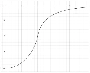
graph for function
𝐹(𝑥) = − ( 1 +1−𝑥2𝑥2ln |1+𝑥1−𝑥|) , we see that it increases monotonously from −2 and
approaches 0 at infinity.
𝑥 = 1 corresponds to 𝑘 = 𝑘𝐹
𝑑𝐹(𝑥) 𝑑𝑥 = (
1 2𝑥2+
𝑥 2) ln |
1 + 𝑥 1 − 𝑥| −
1
𝑥→ +∞ 𝑎𝑡 𝑥 = 1
∫ 𝑥1 2𝐹(𝑥) = 0
−1 2
The calculation for Total Energy of HEG system as ground-state eigenvalue of 𝐻𝐻𝐹 follows
easily
27 𝐸𝐻𝐹 = 2 ∑ [ 𝑘2
2 − 𝑘𝐹
𝜋 (1 +
𝑘𝐹2− 𝑘2 2𝑘𝑘𝐹 ln |
𝑘 + 𝑘𝐹 𝑘 − 𝑘𝐹|)] 𝒌
− 𝑈𝑒𝑥𝑐ℎ𝑎𝑛𝑔𝑒
= 2 ∑ [ 𝑘2 2 −
𝑘𝐹 2𝜋 (1 +
𝑘𝐹2− 𝑘2 2𝑘𝑘𝐹 ln |
𝑘 + 𝑘𝐹 𝑘 − 𝑘𝐹|)] 𝒌
= 2𝑉
(2𝜋)3∫ 𝑑𝑘 4𝜋𝑘2[ 𝑘2
2 − 𝑘𝐹 2𝜋 (1 +
𝑘𝐹2− 𝑘2 2𝑘𝑘𝐹 ln |
𝑘 + 𝑘𝐹 𝑘 − 𝑘𝐹|)] 𝑘𝐹 0 = 2𝑉
(2𝜋)3 4𝜋 [ 1 2
𝑘𝐹5 5 +
𝑘𝐹4
2𝜋 ∫ 𝑥2𝐹(𝑥) 1 0 ] = 2𝑉 (2𝜋)3 4 3 𝜋𝑘𝐹3[
3 5
𝑘𝐹2 2 −
3
4𝜋𝑘𝐹] = 𝑁( 3 5𝜀𝐹−
3 4𝜋𝑘𝐹)
3
5𝑁𝜀𝐹 is the total energy for free electron gas; the correction to it is exchange energy.
Hartree-Fock exchange energy is the same as first-order perturbation of Coulomb
interaction on free electron gas, since Hartree-Fock eigenstates coincide with
non-interacting eigenstates. In literature, energy per particle is often shown as an expression of
average inter-particle distance 𝑟𝑠(43𝜋𝑟𝑠3 = 𝑉 𝑁=
(2𝜋)3 8 3𝜋𝑘𝐹3
) 𝐸𝐻𝐹 𝑁 = 1 2( 2.2099 𝑟𝑠2 −
0.91633 𝑟𝑠 )
This can be shown to be exact in the high density (𝑟𝑠 → 0) limit. It might seem first to be
counterintuitive. Nevertheless, it’s true that at zero temperature fermions behave more like
free particles at high density. At very low densities, they form Wigner Crystals (Drummond,
28
One alarming feature of the Hartree-Fock spectrum is that 𝑑𝜀𝑘
𝑑𝑘 |𝑘=𝑘𝐹 → +∞ . This means
density of states at Fermi wavevector is 0, i.e. there’s an infinitesimal gap for HEG, which is
unphysical as we know the system should be metallic. The divergence of the derivative can
be traced back to∫ 𝑑𝒒 𝑉𝒒 ~∫ 𝑑𝑞1𝑞= ln |𝑘+𝑘𝐹𝑘−𝑘
𝐹|. Had 𝑉𝒒 been 1 𝑉
4𝜋
𝑞2+𝛼2 , which is the Fourier
transform for screened Coulomb (Yukawa) potential 𝑒−𝛼𝑟𝑟 ,
∫ 𝑑𝒒 𝑉𝒒~∫ 𝑑𝑞𝑞2+𝛼𝑞 2 ~ln |
(𝑘+𝑘𝐹)2+𝛼2
(𝑘−𝑘𝐹)2+𝛼2| so there wouldn’t be this divergence. Screening is
29
Chapter 3 Density Functional Theory
Density functional theory (DFT) is a powerful, formally exact theory. In the formulation of
Kohn-Sham DFT(Kohn & Sham, 1965), it tries to use a non-interacting model to mimic the
behavior of many-body system so it shares some similarities with Hartree-Fock. But instead
of having effectively a non-interaction wavefunction like Hartree-Fock, its non-interacting
system aims to produce the same density distribution as the many-body system, for
ground-state properties of the electronic system is uniquely determined by density according to
Hohenberg-Kohn Theorem(Hohenberg & Kohn, 1964). DFT has come to prominence as a
method potentially capable of very accurate results at low cost. In practice, approximations are required to implement the theory, as the exact mapping between density and
ground-state property like energy is unknown. The next small section is the derivation of
Hohenberg-Kohn theorem. Instead of the original derivation of Hohenberg and Kohn, which
was based upon “reduction ad absurdum”, we follow the “constrained search” approach of
Levy(Levy, 1979).
Hohenberg-Kohn Theorem (Density Variational Principle)
According to variational principle, ground state energy can be expressed as
𝐸 = min
Ψ 〈Ψ|𝐻|Ψ〉
30
We can now separate the minimization into two steps. First we minimize over
wavefunctions that yield a given density 𝑛(𝒓)6 :
min
Ψ→𝑛〈Ψ|𝐻|Ψ〉 = minΨ→𝑛 〈Ψ|𝑇 + 𝑉𝑒𝑒|Ψ〉 + ∫ 𝑑
3𝑟 𝑣(𝒓)𝑛(𝒓)
Then we define the universal functional
𝐹[𝑛] = min
Ψ→𝑛〈Ψ| 𝑇 + 𝑉𝑒𝑒|Ψ〉
Finally we minimize over all 𝑁-electron densities 𝑛(𝒓): 𝐸 = min
𝑛 𝐸𝑣[𝑛]
= min
𝑛 {𝐹[𝑛] + ∫ 𝑑
3𝑟 𝑣(𝒓)𝑛(𝒓)}
, where 𝑣(𝒓) is held fixed during the minimization. The minimizing density is then the
ground-state density.
The constraint of fixed particle number 𝑁 can be handled formally through introduction of
a Lagrange multiplier 𝜇:
𝛿 { 𝐹[𝑛] + ∫ 𝑑3𝑟 𝑣(𝒓)𝑛(𝒓) − 𝜇 ∫ 𝑑3𝑟 𝑛(𝒓)} = 0
, which leads to
6 This is one-body density 〈𝜓+(𝒓)𝜓(𝒓)〉 , diagonal part of one-body density matrix. We use 𝑛(𝒓)
31 𝑣(𝒓) = 𝜇 − 𝛿𝐹
𝛿𝑛(𝒓)
, where 𝜇 is to be adjusted until total conservation of particle number is
satisfied ∫ 𝑑3𝑟 𝑛(𝒓) = 𝑁
This equation shows that the external potential 𝑣(𝒓) is uniquely determined by the ground
state density. The functional 𝐹[𝑛], minimized kinetic energy and electron-electron
interaction for a given density, applies to all densities 𝑛(𝒓) which are “𝑁-representable”,
i.e., coming from an antisymmetric 𝑁-electron wavefunction. The functional derivative 𝛿𝑛(𝒓)𝛿𝐹
is defined for all densities which are “𝑣-representable”, i.e., come from antisymmetric
𝑁-electron ground-state wavefunctions for some choice of external potential 𝑣(𝒓)7.
It is straightforward to generalize the derivation for spin-density functional theory: just
replace the constraint of fixed 𝑛 by that of fixed 𝑛↑ and 𝑛↓. There are two practical reasons
to do so:
(1) This extension is required when the external potential is spin-dependent, for
instance if there’s an external magnetic field. (If this field not only couples to
electron spin but also current density, then we must resort to a current-density
functional theory).
7 We’ll not delve into the discussion of 𝑣-representability in this thesis. Interested readers referred
32
(2) Even when external potential is spin-independent, we may still be interested in
physical magnetization (arising from exchange effect).
Kohn-Sham DFT
For a system of non-interacting electrons, 𝑉𝑒𝑒 vanishes so 𝐹[𝑛] reduces to
𝑇𝑠[𝑛] = minΨ→𝑛 〈Ψ|𝑇|Ψ〉
Even though we can search over all antisymmetric 𝑁-electron wavefunctions, the
minimizing wavefunction for a given density will be a non-interacting wavefunction (a single
Slater determinant) for some external potential 𝑉𝑠 such that
𝛿𝑇𝑠
𝛿𝑛(𝒓)+ 𝑣𝑠(𝒓) = 𝜇
, the Kohn-Sham potential 𝑣𝑠(𝒓) is a functional of 𝑛(𝒓). If there were any difference
between 𝜇 and 𝜇𝑠, the chemical potentials for interacting and non-interacting systems of
the same density, it could be absorbed into 𝑣𝑠(𝒓).
Now we define the exchange-correlation energy 𝐸𝑥𝑐[𝑛] by
𝐹[𝑛] = 𝑇𝑠[𝑛] + 𝑈𝐻𝑎𝑟𝑡𝑟𝑒𝑒[𝑛] + 𝐸𝑥𝑐[𝑛]
, where 𝑈[𝑛] is the usual Hartree energy 12∫ 𝑑𝒓𝑑𝒓′ 𝑛(𝒓)𝑛(𝒓′)
|𝒓−𝒓′| . Then our Kohn-Sham potential
has to be
𝑣𝑠(𝒓) = 𝑣(𝒓) +𝛿𝑈𝐻𝑎𝑟𝑡𝑟𝑒𝑒[𝑛]
𝛿𝑛(𝒓) +
33
= 𝑣(𝒓) + 𝑣𝐻𝑎𝑟𝑡𝑟𝑒𝑒(𝒓) + 𝑣𝑥𝑐(𝒓)
The Kohn-Sham method treats 𝑇𝑠[𝑛] exactly, leaving only 𝐸𝑥𝑐[𝑛] to be approximated. This
makes good sense, for several reasons:
(1) We can guarantee 𝑁-representability of 𝑛(𝒓) and 𝑣-representibility for the trivial
case.
(2) 𝑇𝑠[𝑛] is typically a very large part of the energy, while 𝐸𝑥𝑐[𝑛] is a smaller part.
(3) 𝑇𝑠[𝑛] is largely responsible for density oscillations of the shell structure and Friedel
types, which are accurately described by the Kohn-Sham method.
(4) 𝐸𝑥𝑐[𝑛] is somewhat better suited to the local and semi-local approximations than
𝑇𝑠[𝑛].
The price to be paid for these benefits is the appearance of orbitals. If we had a very
accurate approximation for 𝑇𝑠[𝑛] directly in terms of n, we could dispense with the
orbitals and solve directly for 𝑛(𝒓).
Once we know how to form Kohn-Sham potential from density, we can immediately obtain
a set of self-consistent equations since we can solve for the eigenvectors (orbitals) from
which we can compute the density for the next iteration. This set of equations is known as
Kohn-Sham equations through which we can solve for Kohn-Sham orbitals.
[−1
34
We have made the potential’s functional dependence on density explicit and also
generalized the framework to be spin-dependent (the constraint ∫ 𝑑3𝑟 𝑛(𝒓) = 𝑁 is still on
total density 𝑛(𝒓) = 𝑛↑(𝒓) + 𝑛↓(𝒓)).
The self-consistence process can be illustrated by the simple flow chart below.
𝑛(𝒓) → 𝑣𝑠(𝒓) → 𝜙𝑖 𝑠
𝑜𝑐𝑐𝑢𝑝𝑎𝑡𝑖𝑜𝑛
The total energy of the system can be expressed as
𝐸 = ∑ 𝜀𝑖,𝜎 𝑖,𝜎
〈𝑐𝑖,𝜎+ 𝑐
𝑖,𝜎〉 − 𝑈𝐻𝑎𝑟𝑡𝑟𝑒𝑒[𝑛] − ∑ ∫ 𝑑3𝑟 𝑛𝜎(𝒓)𝑣𝑥𝑐𝜎([𝑛↑, 𝑛↓]; 𝒓) 𝜎
+ 𝐸𝑥𝑐[𝑛↑, 𝑛↓]
Hartree energy has been subtracted due to double counting and all exchange-correlation
part of energy in the sum of eigenvalues has been replaced by the correct 𝐸𝑥𝑐.
Once we have a good approximation of exchange-correlation functional 𝐸𝑥𝑐, we can use
Kohn-Sham equations to solve our system at relatively low computational cost compared to
methods of quantum chemistry.
Approximations for Exchange-Correlation Functional
The local spin density (LSD) approximation(Kohn & Sham, 1965) is among the earliest
attempts at approximating 𝐸𝑥𝑐 and it has long been popular in solid state physics.
𝐸𝑥𝑐𝐿𝑆𝐷[𝑛
35
, where 𝑒𝑥𝑐(𝑛↑, 𝑛↓) is the known exchange-correlation energy per particle for homogeneous
electron gas with uniform spin densities 𝑛↑, 𝑛↓.
Many functionals belong to the category of generalized gradient approximation
(GGA)(Becke, 1986, 1988; Lee, Yang, & Parr, 1988; Perdew, 1985; Perdew, 1986; Perdew,
Burke, & Ernzerhof, 1996; Perdew, Ruzsinszky, et al., 2008; Perdew & Yue, 1986; Wu &
Cohen, 2006). They have the form
𝐸𝑥𝑐𝐺𝐺𝐴[𝑛 ↑, 𝑛 ↓] = ∫ 𝑑3𝑟 𝑓(𝑛↑, 𝑛↓, 𝛻𝑛↑, 𝛻𝑛↓)
This is a kind of simple extension of LSD, more widely used in quantum chemistry (e.g. gives
much better atomization energies), but LSD remains the most popular way to do
electronic-structure calculations in solid state physics. Table 1 and Table 2 provide a summary of
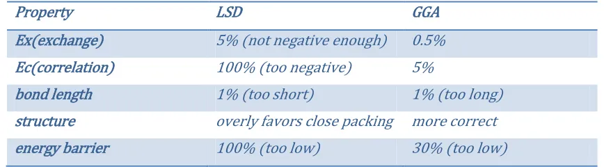
typical errors for LSD and GGA.
The “third-rung” of this “Jacob’s ladder” in exchange-correlation functional approximations
are called meta-GGA (Tao, Perdew, Staroverov, & Scuseria, 2003) which has the general
form
𝐸𝑥𝑐𝑚𝑒𝑡𝑎−𝐺𝐺𝐴[𝑛 ↑, 𝑛 ↓] = ∫ 𝑑3𝑟 𝑓(𝑛↑, 𝑛↓, 𝛻𝑛↑, 𝛻𝑛↓, 𝜏↑, 𝜏↓)
𝜏𝜎 = ∑ |
1
2∇𝜙𝑖,𝜎(𝒓)| 2
𝑖∈𝑜𝑐𝑢𝑝𝑝𝑖𝑒𝑑
Notice that what have been introduced here are merely general mathematical structure
(the more general the mathematical form the higher up in “Jacob’s ladder”). Real
36
Readers should be reminded that Hartree-Fock (introduced in the previous section) treats
exchange exactly, but neglects correlation completely. While the Hartree-Fock total energy
37
Table 1 Typical errors with LSD and GGA approximations
Property LSD GGA
Ex(exchange) 5% (not negative enough) 0.5% Ec(correlation) 100% (too negative) 5%
bond length 1% (too short) 1% (too long) structure overly favors close packing more correct energy barrier 100% (too low) 30% (too low)
Table 2 Mean absolute error of the atomization energies
MAE are for 20 molecules From reference (Perdew, Burke, et al., 1996)
Approximation Mean absolute error (𝒆𝑽) Unrestricted Hartree-Fock 3.1 (underbinding)
LSD 1.3 (overbinding)
GGA 0.3 (mostly overbinding)
38 Coupling-Constant Integration
Following our definition of exchange-correlation functional
𝐸𝑥𝑐[𝑛] = 𝐹[𝑛] − 𝑇𝑠[𝑛] − 𝑈𝐻𝑎𝑟𝑡𝑟𝑒𝑒[𝑛]
= 〈Ψ𝜆 |𝑇 + 𝜆𝑉𝑒𝑒|Ψ𝜆 〉𝜆=1− 〈Ψ𝜆 |𝑇 + 𝜆𝑉𝑒𝑒|Ψ𝜆 〉𝜆=0− 𝑈𝐻𝑎𝑟𝑡𝑟𝑒𝑒[𝑛]
, where we have introduced coupling constant 𝜆 (0 ≤ 𝜆 ≤ 1) and Ψ𝜆 is the wavefunction
that produces the correct density 𝑛(𝒓) while minimizes 𝑇 + 𝜆𝑉𝑒𝑒.
Since Ψ𝜆 is the variational wavefunction within our constraint
〈Ψ𝜆 |𝑇 + 𝜆𝑉𝑒𝑒|Ψ𝜆 〉 ≤ 〈Ψ𝜆′ |𝑇 + 𝜆𝑉𝑒𝑒|Ψ𝜆′ 〉𝜆′≠𝜆
𝑖𝑚𝑝𝑙𝑖𝑒𝑠 → 𝑑
𝑑𝜆′〈Ψ𝜆′ |𝑇 + 𝜆𝑉𝑒𝑒|Ψ𝜆′ 〉𝜆′=𝜆= 0
We can use Hellman-Feynman Theorem to simplify
𝐸𝑥𝑐[𝑛] = ∫ 𝑑𝜆1 0 𝑑 𝑑𝜆〈Ψ𝜆 |𝑇 + 𝜆𝑉𝑒𝑒|Ψ𝜆〉 − 𝑈𝐻𝑎𝑟𝑡𝑟𝑒𝑒[𝑛] = ∫ 𝑑𝜆 1 0 〈Ψ𝜆 |𝑉𝑒𝑒|Ψ𝜆〉 − 𝑈𝐻𝑎𝑟𝑡𝑟𝑒𝑒[𝑛]
This equation “looks like” a potential energy; the kinetic energy contribution to 𝐸𝑥𝑐 has
been subsumed by the coupling-constant integration. We should remember, of course, that
only 𝜆 = 1 is real or physical. The Kohn-Sham system at 𝜆 = 0, and all the intermediate
values of 𝜆, are convenient mathematical constructs.
Now kinetic energy operators are conveniently out of way, we can write the whole
expression in terms various density distributions and Coulomb interaction.
𝐸𝑥𝑐[𝑛] = 1
2∫ 𝑑3𝑟′𝑑3𝑟
𝑛(𝒓)𝜌̅̅̅̅(𝒓, 𝒓𝑥𝑐 ′) |𝒓 − 𝒓′|
𝜌𝑥𝑐
̅̅̅̅ is 𝜆 averaged exchange-correlation hole 𝜌𝑥𝑐𝜆 corresponding to Ψ
39 And exchange-correlation hole is defined such that
𝜌2(𝒓, 𝒓′) = 𝑛(𝒓)(𝜌𝑥𝑐(𝒓, 𝒓′) + 𝑛(𝒓′))
Since 𝜌2(𝒓, 𝒓′) is the two body density define earlier 𝜌
2(𝒓, 𝒓′) =
〈𝜓+(𝒓)𝜓+(𝒓′)𝜓(𝒓′)𝜓(𝒓)〉 , we can see that 𝜌
𝑥𝑐(𝒓, 𝒓′) + 𝑛(𝒓′) is the conditional density
distribution given one particle is already at 𝒓. 𝜌𝑥𝑐 is simply the difference between this
conditional density and 𝑛(𝒓′). 𝑛(𝒓′) is chosen as a reference, for without the effect of
exchange and correlation, particle distribution will be uncorrelated hence 𝜌2(𝒓, 𝒓′) =
𝑛(𝒓)𝑛(𝒓′) and 𝜌
𝑥𝑐 = 0.
It is easy to see 𝜌𝑥𝑐(𝒓, 𝒓′)integrates to −1 over 𝒓′ for a system with fixed number of
particles.
To see this, we can integrate both sides over 𝒓′.
∫ 𝜌2(𝒓, 𝒓′) 𝑑3𝑟′ = (𝑁 − 1)〈𝜓+(𝒓)𝜓(𝒓)〉 = (𝑁 − 1) 𝑛(𝒓)
∫ 𝑑3𝑟′ 𝑛(𝒓)[𝜌
𝑥𝑐(𝒓, 𝒓′) + 𝑛(𝒓′)] = 𝑛(𝒓) [∫ 𝑑3𝑟′𝜌𝑥𝑐(𝒓, 𝒓′) + 𝑁]
Equating both sides, we see
∫ 𝑑3𝑟′𝜌
𝑥𝑐(𝒓, 𝒓′) = −1
Exchange correlation hole conveniently offers intuitive picture of exchange-correlation
effects as “exclusion” of particles at 𝒓′given the presence of a particle at 𝒓.
𝜌𝑥𝑐𝜆 is the exchange-correlation hole of system with interaction coupling strength 𝜆 (𝐻 =
𝑇 + 𝜆𝑉𝑒𝑒)
40 =1
2∫ 𝑑3𝑟′𝑑3𝑟
𝑛(𝒓)𝜌𝑥𝑐𝜆 (𝒓, 𝒓′) |𝒓 − 𝒓′|
The knowledge of 𝜌̅̅̅̅ (𝜆 averaged) would uniquely determine exchange- correlation energy 𝑥𝑐
density
𝑒𝑥𝑐(𝒓) = 1
2∫ 𝑑3𝑟′ 𝜌𝑥𝑐 ̅̅̅̅(𝒓, 𝒓′)
|𝒓 − 𝒓′|
𝐸𝑥𝑐 = ∫ 𝑑3𝑟 𝑛(𝒓)𝑒𝑥𝑐(𝒓)
However, accurate description of exchange-correlation hole is not a mathematically
necessary condition to have a working 𝐸𝑥𝑐. For example, in an inhomogeneous system
exact 𝜌𝑥𝑐 would have various kinds of different shapes (anisotropic), but only the spherically
averaged one would matter to 𝐸𝑥𝑐 as Coulomb interaction is isotropic i.e. we only need
∫ 4𝜋|𝒓−𝒓𝑑2𝑟′′|2 𝜌𝑥𝑐(𝒓, 𝒓′)
|𝒓′−𝒓|=𝑐𝑜𝑛𝑠𝑡𝑎𝑛𝑡 to be correct. For this reason, one often drops the vector
notation for second-electron coordinates and uses a scalar to indicate the distance between
two particles like 𝑢 = |𝒓 − 𝒓′| and use 𝜌
𝑥𝑐(𝒓, 𝑢) to denote the spherically averaged value.
Therefore, normalization for 𝜌𝑥𝑐 amounts to the second moment of hole density
∫ 𝑑𝑢 4𝜋𝑢2𝜌
𝑥𝑐(𝒓, 𝑢) = −1
, and 𝑒𝑥𝑐(𝒓) is nothing other than the first moment of hole density.
𝑒(𝒓) = 1
2∫ 𝑑𝑢 4𝜋𝑢2
𝜌𝑥𝑐(𝒓, 𝑢)
𝑢 = ∫ 𝑑𝑢 2𝜋𝑢 𝜌𝑥𝑐(𝒓, 𝑢)
Thus, if the exact exchange-correlation hole is not too extended, the approximation can’t be