Assessing Complex Genetic Effects Using Variance Component Based Marker-set Methods.

(1)

ABSTRACT

ZHAO, GUOLIN. Assessing Complex Genetic Effects Using Variance Component Based Marker-set Methods. (Under the direction of Dr. Jung-Ying Tzeng and Dr. Daowen Zhang.)

(2)

study data and next generation sequencing data.

(3)

(4)

Assessing Complex Genetic Effects Using Variance Component Based Marker-set Methods

by Guolin Zhao

A dissertation submitted to the Graduate Faculty of North Carolina State University

in partial fulfillment of the requirements for the Degree of

Doctor of Philosophy

Statistics

Raleigh, North Carolina 2013

APPROVED BY:

Dr. Wenbin Lu Dr. Dahlia Nielsen

Dr. Jung-Ying Tzeng Co-chair of Advisory Committee

(5)

DEDICATION

(6)

BIOGRAPHY

(7)

ACKNOWLEDGEMENTS

I would especially like to express my gratitude to my advisors Dr. Jung-Ying Tzeng and Dr. Daowen Zhang for their guidance, patience and encouragement throughout the years working on the research and writing of this dissertation. I greatly appreciate the time and effort that both of them dedicated to helping me complete the research study smoothly.

I would like to thank my committee members Dr. Wenbin Lu, Dr. Dahlia Nielsen and Dr. Jeffrey Thorne constructive comments and suggestions for my research.

I would also like to thank all the Directors of Graduate Programs (DGP) Dr. Pam Arroway, Dr. Jacqueline M. Hughes-Oliver, Dr. Sujit K Ghosh and Dr. John F Monahan. It is their assistance, effort and encouragement to make my graduate study life meaningful. I am also grateful to Dr. Howard Bondell and Dr. Jason Osborne for their guidance on the course work and help on the research work. I am grateful to all the faculty members, staffs, fellow students and friends who I know during the years that ever helped.

In addition, I am grateful to Dr. Timothy Frayling and Dr. William Rayner and members of the Warren 2 Consortium for providing us the BMI data. This work makes use of data generated by the Wellcome Trust Case Control Consortium (WTCCC). A full list of the investigators who contributed to the generation of the data is available from http://www.wtccc.org.uk. I am also thankful to Dr. Michael Wu for helping with the simulation design. I am also appreciative to Dr. Mathieu Firmann and Dr. Vladimir Mayor and members in the CoLaus study for providing the CoLaus study data.

(8)

LIST OF TABLES

Table 2.1 Type I error rates for examining the joint effect over 1000 runs using the COSI based simulation data. . . 29 Table 2.2 Type I error rates for examining the Gene-Environment effect over 1000

runs using the COSI based simulation data. . . 30 Table 2.3 Type I error rates for examining the joint effect over 1000 runs using the

Hapmap based simulation data . . . 31 Table 2.4 Type I error rates for examining the Gene-Environment effect over 1000

runs using Hapmap based simulation data. 4 scenarios are considered where 2 causal SNPs are used under each scenario. For scenario (1), a rare vari-ant and a low frequency varivari-ant are used as the causal SNPs (“RL”). For scenario (2), a rare variant and a common variant are used as the causal SNPs (“CR”). For scenario (3), a low frequency variant and a common variant are used as the causal SNPs (“CL”). For scenario (4), two common variants are used as the causal SNPs (“CC”). The reference SNP ID num-bers are provided corresponding to each causal SNP with its MAF using the Hapmap3 data. . . 32 Table 3.1 The averages and medians of R2 values between the SNPs from two

dif-ferent genes. The numbers without parentheses are the averages and the numbers with parentheses are the median values. . . 49 Table 3.2 The gene identification rates (percents) and the probabilities (percents)

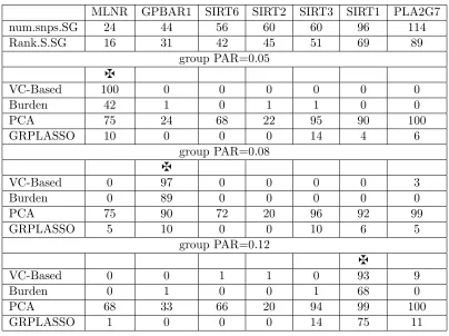
of detecting the false positives over 100 runs when one of the three genes MLNR, GPBAR1, and SIRT1 is used as the causal gene. All the seven genes are assumed to be mutually uncorrelated where we usezto denote the causal gene under each scenario. When MLNR is the causal gene, a group PAR value of 0.05 is assigned to the causal gene. When GPBAR1 is the causal gene, a group PAR value of 0.08 is assigned to the causal gene. When SIRT1 is the causal gene, a group PAR value of 0.12 is assigned to the causal gene. . . 53 Table 3.3 The gene identification rates (percents) and the probabilities (percents)

(11)

Table 3.4 The gene identification rates (percents) and the probabilities (percents) of detecting the false positives over 100 runs when genes MLNR and SIRT1 are used as the causal genes. Different group PAR values of 0.05 and 0.08 are assigned to the two causal genes MLNR and SIRT1, respectively. All the seven genes are assumed to be mutually uncorrelated where we usez’s to denote the two causal genes under each scenario. . . 56 Table 3.5 The gene identification rates (percents) and the probabilities (percents) of

detecting the false positives over 100 runs when all the three genes MLNR, GPBAR1, and SIRT1 are used as the causal genes. All the seven genes are assumed to be mutually uncorrelated where we usez’s to denote the three causal genes under each scenario. A group PAR value of 0.05 is assigned to the three causal genes. . . 57 Table 3.6 The gene identification rates (percents) and the probabilities (percents)

of detecting the false positives over 100 runs when one of the three genes MLNR, GPBAR1, and SIRT1 is used as the causal gene. The LD structure is maintained among the seven genes where we usezto denote the causal gene under each scenario. When MLNR is the causal gene, a group PAR value of 0.05 is assigned to the causal gene. When GPBAR1 is the causal gene, a group PAR value of 0.08 is assigned to the causal gene. When SIRT1 is the causal gene, a group PAR value of 0.12 is assigned to the causal gene. . . 58 Table 3.7 The gene identification rates (percents) and the probabilities (percents)

of detecting the false positives over 100 runs when two of the three genes MLNR, GPBAR1, and SIRT1 are used as the causal genes. The LD struc-ture is maintained among the seven genes where we usezto denote the two causal genes under each scenario. When the pair of MLNR and GPBAR1 and the pair of MLNR and SIRT1 are considered as the causal genes, a group PAR value of 0.05 are assigned to the two pair of the causal genes. When GPBAR1 and SIRT1 are the two causal genes, a group PAR value of 0.10 is assigned to the two causal genes. . . 59 Table 3.8 The gene identification rates (percents) and the probabilities (percents) of

detecting the false positives over 100 runs when genes MLNR and SIRT1 are used as the causal genes. Different group PAR values of 0.05 and 0.08 are assigned to the two causal genes MLNR and SIRT1, respectively. The LD structure is maintained among the seven genes. We use z to denote the two causal genes under this scenario. . . 60 Table 3.9 The gene identification rates (percents) and the probabilities (percents) of

(12)

(13)

LIST OF FIGURES

Figure 2.1 The Eigenvalues and the corresponding cumulative proportions of the total information in the similarity matrix S by using a next-generation sequence data set and a genome-wide association study data set. . . 20 Figure 2.2 The power comparisons for gene-environment test and joint test over 500

simulation runs using the COSI based simulation data. The solid lines are the power by applying the proposed variance component based method. The dashed lines are the power by applying the counting based burden test. 38 Figure 2.3 The power comparisons for gene-environment test and joint test over 500

runs under the three LD-level conditions using the Hapmap based sim-ulation data. In each box-plot, the summary for the power by using the proposed variance component based method (VC-Based) is shown on the left and the summary for the power by using the minimum P-value (min-Pval) approach is shown on the right. A red “X” in each box-plot is the power average under each LD condition. . . 39 Figure 3.1 The Boxplots for theR2 values between each pair of genes. EachR2value

calculates the correlation between two SNPs from different genes. In each boxplot, it present the minimum, first quartile, median, third quartile, maximum and the outliers of the R2 values between two genes. . . 48 Figure 3.2 Plots of BIC scores corresponding to pre-specified log(λ)’s using the

Co-Laus study data. The first plot at the top shows the BIC scores for

(14)

Chapter 1

Introduction

1.1

Genetic Associations of Complex Diseases

(15)

innovative because it is the first time that the skin defense system is demonstrated to be as important as the immune system in allergic pathways [5].

Recent genome-wide association studies (GWAS) have revealed a polygenic basis for complex disorders. Both common and rare variants are involved, and individual genetic effects tend to be moderate due to low individual impact or rarity of the mutation. Numerous methods have been proposed to perform association analysis at gene, protein, pathway or network level. These approaches differ in the way on how the genetic information is aggregated to examine the association. Details are reviewed in the subsequent sections.

1.2

Gene-Level Association Analyses

When multiple single-nucleotide polymorphisms (SNPs) in a gene are genotyped to assess the complex genetic effect, both SNP-based and gene-based analyses could be considered to test whether the gene is associated with the disease.

In SNP-based methods, the effect of each SNP is assessed one at a time. The major tasks in the SNP-based methods are how to combine the individual test results at gene level and how to account for multiple testing. The minimum p-value method [6] and the Fisher’s combined method [7] are commonly used to combine individual test results. To account for multiple testing, the adjusted threshold,α∗_i, are calculated by certain procedures to ensure the family-wise error rate is under control. For example, Bonferroni correction givesα∗_i =α/M, whereM

is the number of SNPs in the gene and α is the family-wise error rate. Sidak correction gives

(16)

Alternatively, gene-based methods that analyze a group of SNPs simultaneously are consid-ered, and these approaches are also referred to as “marker-set” or “multi-locus” methods. Even though each variant may have moderate effect, the overall effect of multiple loci from the gene could be clinically significant. Based on how the genetic information is collapsed across loci, marker-set methods can roughly be categorized into two types [8]: genotype collapsing methods and similarity collapsing methods.

Genotype collapsing methods combine the multi-locus information by first obtaining a weighted or unweighted sum of the individual genotypes across markers, and then assess the multi-locus effect based on the genotype sum. For example, PCA-based methods [9, 10] compute the principal components (PCs) of the genotypes and then use the PCs to assess the associa-tion between the disease trait and the genetic informaassocia-tion. In rare variant analysis, due to the sparseness of mutations, the “newer” generations of genotype collapsing methods incorporate the minor allelic frequencies in the weights [11, 12, 13]. Specifically, these approaches aim to assess the overall genetic burden due to rare variants, which are in essence weighted genotype sums. Methods of this type, such as the counting based burden test (sum test) [14] and weighted sum test [12], implicitly assume all the variants affecting the disease risk in the same direction and thus may lose power when the assumption is violated [15, 16, 17]. The genotype collapsing methods are recommended when additive genetic effects with similar effect size are present among the markers [8].

(17)

The kernel machines-based methods [18, 25, 27, 19, 20, 17, 28] incorporate the pairwise genetic similarity via kernel functions. Some commonly used kernel functions include (a) the identity by state (IBS) kernel [29], which is the number of alleles shared by state and is rec-ommended when nonlinearity or interactive effect is present; (b) the linear kernels [19, 30], which offers higher power if only linear additive effect is present among the SNPs [28]; and (c) the polynomial kernel, which is considered when SNPs within a small window have local correlations due to linkage disequilibrium (LD) but no long-range correlations among the SNPs [27].

The idea of the gene-trait similarity regression[21, 22] is inspired by Haseman-Elston re-gression [31] from linkage analysis and haplotype similarity tests [32] for regional association. It takes pairs of individuals and regresses their trait similarity on genetic similarity of a marker set. If the markers are associated with the trait, the slope should be non-zero.

Finally, the random effect methods [23, 24] incorporate genetic similarity information into the variance-covariance structures of the genetic effects. The gene-trait associations could be studied by testing the variance components in these random effect models.

Compared to the genotype-collapsing methods which detect the association by examining the mean genetic effects, similarity collapsing approaches detect the association by examining the variance of the genetic effects. Similarity collapsing methods have higher power when non-linear or interactive effects are present among markers with different effect sizes and are more robust under complex genetic architectures [8].

1.2.1 Connections among different similarity-collapsing methods

(18)

Consider a GLMM which includes fixed covariates effect and genetic random effect:

g(µ) =Xγ+G, (1.1)

where g(·) is the link function connecting the conditional mean vector µ of the complex trait vector Y and the explanatory variables or covariates, which forms the design matrix X with coefficient vector γ, and G∼N(0,ΣG) is the matrix of genetic effects forN individuals in the sample where ΣGis aN×N nonnegative definite variance-covariance matrix which incorporates the genetic information.

If one setsGiash(gi1, . . . , giM) for some function, wheregim, m= 1,· · ·, M are the genotypes of locusmfor the individualiand ΣG=τ KwhereK is defined using different kernel functions (e.g., linear kernel or weighted IBS kernel [19, 20]), then the test ofH0 :τ = 0 is equivalent to examining H0 :h(g) = 0 in the kernel machines regression whereg includes all the genotypes forN individuals onM loci [18, 19].

The gene-trait similarity regression model is given as

E(Tij|X, S) =c×Sij, i6=j,

whereTij is the trait similarity for individualsiandj andSij is the pairwise genetic similarity. If one sets Tij as the weighted covariance between Yi and Yj and lets ΣG in Equation (1.1) be specified as τ S with S = {Sij}, then it can be shown that E(Tij|X, S) ≈ τ Sij using the optimal weights determined by the distribution of trait vectorY in calculating the conditional trait similarity expectations. Thus, the variance-component testH0 :τ = 0 is equivalent to the significance test of the regression coefficient in the gene-similarity regression, i.e., H0 : c = 0 [21].

(19)

the similarity between different haplotypes, then the variance component test of H0 :τ = 0 is equivalent to haplotype-based association test proposed in Tzeng and Zhang [24].

With the connections between variance-component based methods and the similarity col-lapsing methods, we see the variance component based methods cover a range of similarity-based approaches, and the key lies in how the variance-covariance structure, ΣG, is specified. The similarity based methods have been shown to have superior power when genetic variants have nonlinear effects with various effect size [8]. In addition, the variance component based methods have well-established theoretical foundation and flexibility in inference. Thus, such con-nection between these two types of methods makes the variance component based approaches as attractive analytical tools for associations.

1.2.2 Methods for testing Gene-Environment Interaction

For multi-factorial complex disorders, gene-environment interaction (GxE) studies can facili-tate the understanding of genetic heterogeneity under different environmental exposures [33, 34]. They help to identify high-susceptible subgroups in the population [35], provide insights into biological mechanisms for complex diseases [35, 36, 37], and improve the ability to discover sus-ceptible genes that interact with other factors but exhibit little marginal effect [37]. In the post genome-wide association studies (GWAS) era, genome-wide GxE studies are undertaken to mine the existing GWAS data, with an aim to uncover the missing inherited risks. In pharmacoge-netics, gene-by-treatment analyses are conducted to understand the inter-individual variations in drug responses, with an aim to suggest personalized prevention, detection and treatment regimes.

(20)

standard SNP-based approaches to test the associations. Modifications are developed based on the classical SNP-methods for case-control study to correct the biases caused by the violations for the assumptions of either independence between gene-environment factors or Hardy Wein-berg Equilibrium (HWE) [39]. Such modifications include adapting logistic regression models with some quadratic penalization [40], and applying an empirical Bayes method to derive a shrinkage estimator [39] under a semiparametric maximum-likelihood framework [41].

There are limitations with the SNP-based approaches. One major issue, as what encoun-tered in the main-effect tests, is the correlations among SNPs. In the analysis testing for the GxE interaction, the multiple tests for SNP-environment interactions could be more dependent because the same environmental effect is shared in the interaction terms under each hypothesis [42]. Potential efficiency loss is another challenge if a large amount of SNPs are present. Thus, marker-set methods could be considered as a better alternative for GxE tests in presence of multiple SNPs.

The same two major types of collapsing methods, genotype collapsing and similarity col-lapsing, can be applied to test the GxE interaction. Several genotype collapsing methods testing for the GxE interactions are simply the extensions for the same type of methods testing for the genetic main effects. In addition, new approaches are also developed for assessing the in-teractions, such as the approach incorporating all the genotypes into a latent variable. Then the interaction is tested under Tukey’s 1 degree-of-freedom models where the latent variable interacted with the environmental exposures [43].

(21)

corresponding variance component.

In addition, methods under Bayesian frameworks are also developed for examining the GxE effects such as a resampling-based test which identify a latent genetic profile variable to classify the genotypes into different clusters such that individuals sharing the same genetic profile category share the same risk model [38].

1.2.3 Topics Addressed in This Dissertation

In Chapter 2 of this dissertation, we developed variance component based methods for examin-ing the GxE effects on binary traits, commonly encountered traits in genetic applications. While methods exist for testing the genetic main effects on binary traits [21] or for testing GxE effects on quantitative traits [22], the direct extensions to GxE binary traits is not straightforward. There are several challenges with respect to computational and estimation issues especially with large sample data.

First, the GxE effect is assessed by testing a variance component corresponding to the GxE effects. Most commonly used methods for hypothesis testing, such as the Wald test and the likelihood ratio test, are not valid under this situation because the variance components to be tested are on the boundary of the parameter space. To conquer these challenges, we consider score-type of test statistics for assessing GxE interaction since score statistics usually have stable statistical properties when the variance component tested at the boundary points.

Second, when assessing the GxE effect using a score statistic, there exists one nuisance variance component that corresponds to the genetic main effect and needs to be estimated under H0. For binary traits, the estimation procedure involves a high-dimensional integration that lacks a closed form. To obtain an acceptable variance component estimate, we propose an approximate EM algorithm to estimate the nuisance variance components and other model parameters.

(22)

large samples. To overcome this problem, we considered matrix decompositions in modifying the proposed generalized linear mixed model where the majority of the information is still maintained. Then the proposed approximate EM algorithm proceeds for the reduced GLMM.

1.3

Gene-Set Association Analyses

Because genes function together within biological modules such as pathways and networks, demands in the methodological development of association analyses have shifted from SNP level and gene level to gene-set level in order to facilitate understanding of the biological mechanisms for complex diseases. Gene-set association analyses (GSAA) evaluate the significance of a pre-defined gene set (such as a biological pathway) with the trait values. Gene-set analyses were once primarily applied on the gene expression studies [44, 45, 46, 47, 48, 49, 50] and have now been widely used as a complementary tool to mine GWAS data.

There are two types of statistical hypotheses evaluated under GSAA: the competitive hy-potheses and the self-contained hyhy-potheses. A null hypothesis is a competitive one if we examine the association from a gene-set compared to other genes that are not in the pre-defined set. The well-received ALIGATOR (Association LIst Go AnnoTatOR) [51] is a representative com-petitive test for gene-set analyses. Our focus is on the self-contained tests. The null hypothesis is self-contained if it examines whether genes from the pre-defined gene-set have significant effect on the trait values [52]. Methods such as gene-set ridge regression in association stud-ies (GRASS) [53] and supervised principal component analysis (SPCA) [54] are self-contained tests.

(23)

regularized regression [53]. Because of the unnecessary relation between the eigenSNPs and the phenotypes, SPCA is proposed which identifies significant genes using principal components incorporating the correlations between SNPs [54].

1.3.1 Variable Selection Methods for Testing Gene-Set Associations

To identify the genes associated with a disease under the self-contained hypothesis, many vari-able selection techniques can be applied to identify the significant disease-associated genes. These methods can be roughly classified into two types.

The first type is the grouped variable selection based methods, which treat genetic informa-tion within same gene as a group of variables. Regularizainforma-tion methods such as Group-LASSO [55, 56, 57] and group ridge regression [58] could be applied either directly on the SNPs data or on the principal components of multi-locus genotypes within each gene. GRASS is such a method in which a group ridge penalty is imposed to shrink the estimates of the genes and a lasso penalty is used to perform variable selection on the eigenSNPs within each gene [53].

The second type is the individual variable selection based methods such as stepwise selection, LASSO [59] and adaptive LASSO [60] in which genetic information within each gene is either summarized in one variable or corresponded to one variance component. Such gene-specific variables could be obtained by using genotype collapsing methods, such as the counting based burden methods using a single count to represent a single gene. Regularization penalty terms could also be imposed on gene-specific variance components, the proposed variance component based method introduced in this research work is such an example.

1.3.2 Topics Addressed in This Dissertation

(24)

within each gene in an efficient way. In addition, due to the modest genetic effect and LD among the SNPs, another challenge in GSAA is to identify the disease-associated genes with subtle genetic effects but significant overall multi-gene effects [53, 54, 61].

(25)

Chapter 2

Association Tests for

Gene-environment Interaction on

Binary Traits using Generalized

Linear Mixed Models

2.1

Introduction

(26)

changing the modifiable environment [37].

Hundreds of genes have been identified to be significantly associated with multi-factorial dis-orders by using numerous single-SNP methods developed for genome-wide association studies. Such discoveries encourage researchers to continue their contributions in exploring the under-lying genetic and environmental effects associated with complex diseases. Even though it was a great success brought by those single-SNP methods in GWAS, there are even larger part of the trait heritability is remained unexplained and undiscovered [64]. To explore more proportion of trait heritability, approaches assessing the association on multiple markers may be of desire because genetic variants may function together and confer the disease risk at different genetic levels simultaneously. Thus, the overall effect of these variants is more possible to be significant in detecting the association between the complex disease and traits if aggregating at the correct level [65].

With the development of resequencing technology, thousands or millions of rare variants are genotyped. These rare variants may have subtle effects individually or occur sparsely which have a more recent origin [66]. According to this fact, rare variants should not be ignored in association analyses for complex diseases. Due to the sparse mutations, significance is barely detected by using the single-SNP methods in the presence of rare variants. Additionally, these methods mostly ignore the correlation among the markers, which may lead to the consequence that the LD structure for the markers is automatically not taken into account. Therefore, multi-locus approaches are considered as major methods in association studies for genetic variants with low minor allele frequencies.

(27)

are often lack of replications by using the single-SNP methods. Abundant marker-set methods have been proposed for genetic main effect analyses to enhance detecting power [8], and we argue that the same strategies should be considered for GxE studies. First, GxE with G being genes, pathways or functions, provides a biologically sensible way to assess jointly whether the gene/pathway effects are modified under different environmental exposures. Second, assessment of the effect G, E and GxE individually often requires large number of parameters, and when the analyses are conducted at gene or pathway level, the dimensionality is even higher. In contrast, marker-set methods are able to perform efficient analysis by summarizing high dimensional information using smaller number of parameters and by aggregating moderate signals across multiple factors. Therefore, analyses using the information based on a marker-set should be advocated and be developed for examining the GxE interaction where multiple markers and environment factors are presented to cause the complex diseases. It is also the reason that analyses based on marker-set have drawn attention in GWAS and next generation sequencing research studies [8]. Attracted by these advantages, several methods have been developed by applying the similarity collapsing technique which included the kernel machine approaches [18, 19, 20] and similarity-based approaches [22, 21].

(28)

the models. Though the same problem is also present for quantitative traits, such problem is bypassed by the properties of the normal distribution. In models where the genetic main effect is of interest with no GxE interaction, only fixed effects are in the model under the null hypothesis. Thus, there is no need to estimate the nuisance variance components when testing the genetic main effect. In that situation, a generalized linear model such as the logistic linear regression model is sufficient to estimate the coefficients for the fixed effects in order to compute the test statistic. Similarly, when the genetic main effect and gene-environment interaction effect are both of interest, the problem will also simplify because there is no nuisance parameters in the model under the null hypothesis. Second, in order to estimate the variance component, a high dimensional integration may be involved where in cases it is impossible or extremely complicated to derive the integration. To avoid such a trouble, we use the approximate EM algorithm to approximate the integration. Third, most common methods testing the association, such as the Wald test and the likelihood ratio test, are not valid under the situations where variance components are tested at its boundary of the parameter space.

(29)

2.2

Material and Method

2.2.1 Generalized Linear Mixed Model for Gene-Environment Effect

Generalized linear mixed models are not specifically developed for association tests, but more and more studies have shown the power by using the GLMM framework. Even though only few studies have directly proposed the generalized linear mixed models for association studies [24], those variance component based models have been shown to have the connection with various methods [19, 25, 26, 20]. For example, the connection between GLMM and similarity collapsing methods shows that the genetic similarity information among individuals could be incorporated into the variance-covariance matrix for the random effects in the GLMM. By showing the equivalence, we could take the benefit from both types of methods. The similarity collapsing method could gain power when the genetic variants have nonlinear effects with diverse effect sizes, and the generalized linear mixed models have a systematic theoretical foundation and flexibility in inference.

In this work, we propose a generalized linear mixed model incorporating both the genetic main effect and gene-environment effect to assess the gene-environmental interaction. This work is motivated by the previous research by Tzeng and Zhang [24] in which they proposed a generalized linear mixed model using the haplotype information. In the proposed GLMM, the genetic information could be either haplotype information or genotypes from a market-set. It is an extension work with a generalized form of the variance component based model that has been proposed for the quantitative traits [22]. In this work, score tests are conducted on the variance components to examine either the GxE interaction or joint effect.

(30)

X_CiT be theKC×1 design vector for the confounders andKC is the number of such covariates. Environmental factors are not used for assessing the gene-environmental interactions are all included in the confounder vector. Let X_iT = (1, X_CiT , X_EiT ) be a (KC+KE + 1)×1 covariate vector which includes the intercept. All covariates are standardized to mean 0 and variance 1. Let γ be the coefficient vector for the intercept and covariates. Let D be a N ×N diagonal matrix with covariate of environment effect on its diagonal (i.e. Dii =XEi for i= 1, . . . , N). LetGbe the random effects containing the genetic main effects andηbe the random effects for the genetic effect in the GxE interaction. Letµ= (µ1, . . . , µN) be the vector of the conditional means where each conditional mean µi = E(Yi|X, S, G, η). Let S be the similarity matrix where each element calculates the genetic similarity between two individuals. There are several approaches to characterize the similarity [18, 29]. Suppose either haplotype or genotypes atM

loci (plural of “locus”) are known, let g_im for i = 1, . . . , N and m = 1, . . . , M be the genetic information for individual i at locus m. We value g_im = 0 if the genotype at a single locus is homozygous for minor alleles,g_im= 1 if the genotype is heterozygous, andg_im= 2 if the genotype is homozygous for major alleles. To calculate the genetic similarity for individual iand j, we compute the number of alleles they share purely by state at each locus, denoted asIBS(g_im, g_jm) [29]. That isIBS(gm_i , g_jm) = 0 if both individuals are homozygous at locusmwith different SNP alleles (e.g. g_im =AA and g_jm =aa), IBS(gm_i , gm_j ) = 1 if they share one allele (e.g. g_im =AA

and gm_j =Aa), andIBS(gm_i , g_jm) = 2 if they are both homozygous with the same alleles (e.g.,

gm_i =AAandgm_j =AA). In this work, similarity based on identity-by-state (IBS) allele sharing (S_ijIBS) and similarity based on weighting by allele frequency (S_ijW) are applied. The former similarity is defined as S_ijIBS = PM

m=1IBS(gim, gmj )/2M. The latter similarity is defined as

S_ijW =PM

m=1wmIBS(gmi , gjm)/

PM

(31)

calculates the unweighted similarity and S_ijW calculates the weighted similarity incorporating the minor allele frequency information. In cases where almost all variants are common alleles, the unweighted similarity S_ijIBS could be considered. In the presence of rare alleles, S_ijW is preferred because it is believed that individuals who share rare alleles are more likely to share similar genomes and thus the weighted similarity might improve the power for detecting variants significantly associated with the phenotypes [29].

To illustrate the generalized linear mixed model, we considerKE = 1 but the proposed work can be extended straightforwardly toKE >1. Thus, the proposed GLMM is expressed as

g(µ) =Xγ+G+Dη, (2.1)

whereG∼N(0, τ S) andτ is the variance component corresponding to the genetic main effect;

η ∼ N(0, φS) and φ is the variance component corresponding to the GxE effect; and g(.) is the link function specified as the logit of µi under the binary cases which is expressed as

g(µi) =logit(µi) = log{µi/(1−µi)}.

However, because of the high dimensional calculation with respect to the N×N similarity matrixS, we rewrite the Model (2.1) in a different form in order to make it more computationally efficient by reducing the dimension. All the further tests on the variance components will be conducted by applying the following model

g(µ) =Xγ+Zb+DZλ, (2.2)

where Z is a N ×L matrix such that ZZT =S, b ∼ N(0, τ I), λ ∼N(0, φI), I is the L×L

(32)

applied on the similarity matrix such thatS = ΣL_l₌₁υlelelT whereυ1 ≥υ2 ≥. . . υL≥0 are the eigenvalues ofS in decreasing order andel’s (l= 1, . . . , L) are the corresponding eigenvectors. The matrix Z is then formed as Z = [√υ1e1, . . . ,

√

υLeL] which leads to ZZT =S. In order to reduce the dimensionality ofZ, we identify ap∈(0,1). For thisp, there exists a minimum value ofL∗ such that ΣL_l₌₁∗ υl/ΣL_l₌₁υl≥p. With an appropriate choice ofp, ˜S = ΣL

∗

l=1υleleTl could hold the most important information and thus to approximate to the original similarity matrix S. Consequently, we denote ˜Z= [√υ1e1, . . . ,

√

υLeL∗] such that ˜ZZ˜T = ˜S. Thus, we expect the ˜Z

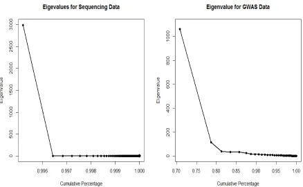
replaced in the Model (2.2) to solve the high dimensionality problem. To investigate the patterns for the two types of data, next generation sequencing data and GWAS data, Figure 2.1 shows eigenvalues and cumulative percentages of the information explained by the first several leading eigenvalues. We could observe that for next generation sequencing data where most alleles are rare variants, the first eigenvalue could explain as high as 99.6% of the total information. On the contrary, we need much more eigenvalues to explain up to 99% of the information for GWAS data. Therefore, in this research study, the principal component technique will be considered for next generation sequencing data in the presence of rare variants.

Under Model (2.2), it is straightforward that the GxE interaction can be examined by testing the null hypothesis of H0 :φ = 0. Although the main focus of this work is to test the interaction effect of gene and environment, a test examining the “joint effects” of genetic main effect and gene-environment interaction effect simultaneously is also covered. We use the term “joint test” to represent the score test examining the joint effects for the null hypothesis of

(33)

Figure 2.1: The Eigenvalues and the corresponding cumulative proportions of the total infor-mation in the similarity matrixS by using a next-generation sequence data set and a genome-wide association study data set.

2.2.2 Connection between the Generalized Linear Mixed Model and a cor-responding Gene-Trait Similarity Regression Model

Motivated by the previous work showing the connection between the variance component models and gene-trait similarity regression models [22, 21], we want to show that examining the variance components in Equation (2.1) is equivalent to testing the GxE effect and the joint effect in a gene-trait similarity regression model.

(34)

E(Tij|X, S) =c×Sij +d×Sij×XEiXEj, i6=j, (2.3)

where Tij is the trait similarity for individuals iand j using the weighted covariance between

Yi and Yj. Specifically, Tij = {ωi(Yi −µ0i)}{ωj(Yj −µ0j)} [21], where µi0 = E(Yi|Xi, Si.) is the subject-specific trait mean accounting for the covariates but assuming no genetic effects. For binary phenotypes, we consider a logistic model that regresses the binary traits on the covariates such thatµ0_i =eXiγ_/_{(1 +}_eXiγ_{). Quantity}_ω

i is a pre-specified weight to account for the unequal variance ofYi. In this work, we use the optimal weight based on the logistic model, i.e., ωi = 1/µ0_i(1−µ0_i) [21].

As indicated above, we consider one environmental effect interacting with the gene effects in this work, which implies that XEi and XEj in the Model (2.3) are scalars. In Model (2.3),

Sij could be either unweighted similarity SijIBS or weighted similarity SijW defined in Section 2.2.1. Due to the reason of the standardization in Tij, there is no intercept and interaction of the two covariates XEiXEj [22]. Under the Model (2.3), the GxE effect is examined under the null hypothesis of H0 :d= 0 and the joint test could be conducted under the null hypothesis of H0 :c=d= 0.

Under the Model (2.1) for binary cases, we assumeYi to be conditionally independent with the conditional meanµi =δ(Xiγ+Gi+XEiηi) whereδ(.) =g−1(.), variancevar(Yi|X, S, G, η) =

µi(1−µi). Taking the Taylor expansion on mean function µi = g−1(Xiγ +Gi+XEiηi) with respect toGand η around E(G) = 0 and E(η) = 0 respectively, we show that

E(Yi|X, S) = EG{Eη(µi|X, S, G, η)}

≈ EG{Eη(g−1(Xiγ +Gi) + [g0(Xiγ+Gi)]−1XEiηi|X, S, G, η)} = EG{g−1(Xiγ+Gi)|X, S, G}

≈ EG{g−1(Xiγ) + [g0(Xiγ)]−1Gi|X, S, G} = µ0_i.

(35)

Because of the approximation shown in Equation (2.4), we thus derive the approximation for the covariance ofYi and Yj under the GLMM which is expressed as

cov(Yi, Yj|X, S) = E[{Yi−E(Yi|X, S)}{Yj−E(Yj|X, S)}|X, S]

≈ E[(Yi−µ0i)(Yj−µ0j)|X, S].

As a result, the expectation of the gene-trait similarity Tij conditional on X and S is approximate to the quantity shown as follows

E(Tij|X, S) = E[{ωi(Yi−µ0i)}{ωj(Yj−µ0j)}|X, S]

≈ ωiωj ×cov(Yi, Yj|X, S)

≈ ωiωj ×[g0(Xiγ)g0(Xjγ)]−1{τ Sij +φXEiXEjSij}.

(2.5)

The details of the derivation shown in Equation (2.5) are provided in Appendix A. If we choose

ωi =g0(Xiγ) as the weight, the expected gene-trait similarity E(Tij|X, S) could be expressed as

E(Tij|X, S)≈τ Sij +φXEiXEjSij.

It is straightforward that the E(Tij|X, S) derived from the generalized linear mixed model shown in Equation (2.2.2) is equivalent to the Model (2.3). Thus, testing the coefficients in the gene-trait similarity regression model given in Equation (2.3) is equivalent to examining the variance components in the generalized linear mix model shown in Equation (2.1).

2.2.3 Score Test

Under the proposed generalized linear mixed model, the score test to examine GxE effect could be derived as [72]

UGxE= 1 2{(y

W ₋_X_ˆ_γ₎T_V−1 0 ΣV

−1 0 (y

W ₋_X_ˆ_γ₎₋_tr₍_P_0Σ)_}|

(36)

where yW is the working vector calculated by yW = Xγˆ+Zˆb+ ∆(y−µˆb) under the model assuming no GxE interaction effect in it and Σ =DSD. Under the same assumption, g(µ) =

Xγ +Zb, ∆ = diag{g0(µi)} with g0(µi) = 1/{µi(1−µi)}, V0 = W−1 +τ S where W =

diag{µi(1−µi)} and P0 =V0−1−V −1

0 X(XTV −1

0 X)−1XTV −1 0 .

Similarly, the score test which examines the joint effect of both gene and gene-environment effects is represented as

Ujoint = 1 2{(y

∗W ₋_X_ˆ_γ₎T_V∗−1 0 Σ

∗_V∗−1 0 (y

∗W ₋_X_ˆ_γ₎₋_tr₍_P_0Σ∗₎_}|

φ=0,τ=0,γ=ˆγ, (2.7)

where y∗W ₌_X_γ_ˆ_{+ ∆(}_y₋_µ_ˆ0_{), Σ}∗ ₌_DSD₊_S _and _V∗

0 =W−1. The details of estimating the fixed effects and variance components are given in Appendix B. The details in computing the test score statistics, their corresponding distributions and p-values calculation are provided in Appendix C.

In cases when variants are common such as in the simulation on Hapmap based data and real data application on GWAS data, the unweighted similarity matrix SIBS is considered. In cases of multiple rare variants are present such as in the simulation on COSI based data and real data application on CoLaus data, the weighted similarity matrixSW is preferred.

2.2.4 Simulation Studies

(37)

similarity matrixSIBS was considered.

Simulation Study using the COSI Based Data

In the simulation study for COSI based data, the haplotype information was provided on 10,000 chromosomes, where 1Mb region on each chromosome was generated according to a coalescent model where the LD pattern and population history was mimicked by using COSI [20]. Genetic variants with minor allele frequency less than 5% are defined as “rare variants” and the first 100 rare variants were chosen from the 1Mb region and used in the analysis. The simulation study was conducted based on the haplotype information from the variants in the gene bank.

We used the logistic model shown in Equation (2.8) to generate the COSI based data

logit P(Yi= 1|Xi, G) =γ0+XEiγE+G1iγG1 +· · ·+GRiγGR+G1iXEiγGxE1 +· · ·+GRiXEiγGxER , (2.8) whereG1i, . . . , GRiare the genotype information of the firstRrare variants selected as the group of disease-risk contributing variants (D-variants) from the gene bank. We also used “causal SNPs” to indicate these D-variants in this article exchangeably.

In the Equation (2.8), the coefficients γ_G1, . . . , γ_GR for these R D-variants were computed as

γr_G= log

αG (1−αG)qr

+ 1

, r= 1, . . . , R,

where qr is the minor allele frequency for rth variant based on the haplotype information of 10,000 simulated chromosomes andαG is the marginal population attributable risk (PAR) for gene effect which controls the low marginal effect on each rare SNPs [12]. The coefficients for each gene-environment effectγ_GxE1 , . . . , γ_GxER in the same Equation were assigned as

γ_GxEr = log

αGxE (1−αGxE)qr

+ 1

, r= 1, . . . , R.

(38)

variant a coefficient using a same marginal PAR (α) to make sure the low effect for each variant. Therefore, we calculated the marginal PAR for gene main effect as αG = group-PARG/R. Without loss of generality, group-PAR_G= 0.02 throughout this simulation study for the COSI based data. Similarly,αGxE = group-PARGxE/Rwas defined as the marginal PAR for each GxE effect. In this simulation study, group-PAR_GxE= 0.1 was applied for the COSI based data.

For simplicity, no confounders are included in the models for this stimulation study and only one environmental effect was included in the models. To calculate the similarity based on the genotype information, 2 haplotypes were randomly selected from the gene bank each time which then determined an individual’s genotype.

When testing the power of GxE effect and joint effect, Model (2.8) was applied to generate the simulation data. However, before carrying out any further tests and comparisons, we needed to test if the proposed method controlled the type I error rate in a proper manner for the COSI based data. Both the random sample simulation data and the case control simulation data were generated under the two reduced logistic models based on Model (2.8) respectively. Under the null hypothesis H0 : φ = 0 which assumes no GxE effect but having gene effect, the reduced model is

logit P(Yi = 1|Xi, G) =γ0+XEiγE+G1iγG1 +· · ·+GRiγGR.

Under the null hypothesis H0 : τ = φ = 0 assuming there are no gene and GxE effects simultaneously, the reduced model is

logit P(Yi = 1|Xi) =γ0+XEiγE.

(39)

set, the same three models were used to generate the data until we obtained N/2 cases in the simulated data. To investigate the type I error controlling issue and conduct the power comparison for both study designs, 5 groups of D-variants were tested. The 5 considered groups were the first 20, 40, 60, 80, and 100 variants selected as the groups of D-variants. In addition, situations where 20, 40, 60, or 80 variants were randomly selected as the groups of D-variants were also tested for validation of type I error and conducted for power comparisons. We only showed the results where the first 20, 40, 60, 80, and 100 variants were selected as the groups of causal SNPs in this article, because the results from the other situations are very similar to the results where the firstR variants were selected as D-variants. In this simulation study, the counting based burden test [15, 20, 73] was used as a comparison to the proposed method. The counting based burden test use one “super-variant” which contains all the genotype information from each individual [14]. Then the information for this super-variant was applied to test for either the GxE effect or the joint effect based on the logistic model logit P(Yi = 1|Xi, G) =

γ0+XEiγE+GCiγC+XEiGCiγCE whereGCi is the genotype information of the super-variant for individuali,γC is the fixed effect coefficient corresponding toGCi andγCE is the fixed effect coefficient for the interaction of XEiGCi.

Simulation Study using the Hapmap Based Data

(40)

causal SNPs were assumed to increase the disease risk for practical purpose in the simulation, it had no impact on the direction to affect the risk in real studies.

The following logistic model shown in Equation (2.9) was used to generate the Hapmap based simulation data

logit P(Yi = 1|Xi, G) =γ0+XEiγE +G1iγG1 +G2iγG2 +G1iXEiγGxE1 +G2iXEiγGxE2 , (2.9)

whereG1i and G2i are the two causal SNPs selected from the 29 SNPs. Without loss of gener-ality, we setXEi∼N(0,6), γ0 =−2.5,γE =log(1.5) = 0.4055, γG1 =γG2 = log(1.2)/2 = 0.0912 and γ1

GxE =γGxE2 = log(1.055)/2 = 0.0268.

In this simulation, we considered a same sample size of N = 1500 with N/2 cases andN/2 controls. Using the formula shown in the (2.9), a random sample with around 30% cases was generated. In order to obtain 50% cases for Yi = 1, such model was used to generate the data until we obtained N/2 cases in the simulated data. For each scenario, 2 SNPs were chosen to be the causal SNPs. Therefore, there were 29₂ = 406 scenarios considered and 100 data sets were generated for each scenario to test the power. The power rates were grouped into three categories based on the LD values under each scenario where the LD values were categorized into one of the three conditions: low-LD, median-LD and high-LD structures. The three LD levels were defined based on the empirical values of LD where each LD value was defined as the average of all R2 values under each scenario. Each R2 number was calculated as the LD between an observed marker and a risk locus. Because the causal SNPs were excluded, there were 27 observed markers. Each of the 27 SNPs was used to calculate theR2 with either of the 2 causal SNPs, thus 54 R2 values were computed under each scenario for this study.

(41)

reduced model to generate the data is

logit P(Yi = 1|Xi, G) =γ0+XEiγE+G1iγG1 +G2iγ2G.

Under the null hypothesis ofH0 :τ =φ= 0, the reduced model is

logit P(Yi = 1|Xi) =γ0+XEiγE.

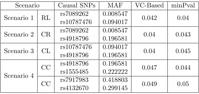
Because there is one rare variant and one low frequency variant among the 29 SNPs, 4 scenarios were tested to investigate the type I error rates. The 4 scenarios are: (1) The two causal SNPs are the one rare variant and the low-frequency allele, denoted as “RL”; (2) one causal SNP is the rare allele and the other SNP is a common allele, denoted as “CR”; (3) one causal variant is the low frequency variant and the other causal SNP is a common allele, denoted as “CL”; (4) both causal SNPs are common alleles, denoted as “CC”. To assess the type I error rates affected by rare or low-frequency alleles with different minor allele frequency (MAF) values, we used the same SNP rs4918796 as the common allele for the scenarios (2) and (3). When testing the association under each scenario, the test statistic and the corresponding p-value were calculated based on the data set excluding the 2 causal SNPs. The motivation of testing GxE effect under 4 scenarios is to verify whether rare or low-frequency alleles deflate the type I error rates for binary traits as which was observed for quantitative traits [22]. Among the 29 SNPs, rs7089262 is the rare allele with MAF of 0.0085, rs10787476 is the low-frequency allele with MAF of 0.0940. The other 27 genotyped SNPs are all common alleles with MAF>0.1. In scenario (4), two pairs of SNPs were randomly selected from the 27 common alleles. As a result, the SNPs rs4918796 and rs1555485 were one pair, and the SNPs rs7917983 and rs4132670 from another pair.

(42)

independent tests to control the overall type I error rate and make the p-value adjustments. The adjusted p-value was computed via the formula 1−(1−minimum p-value)kef f _where_k

ef f the number of independent LD tests [6]. In the simulation study, each of the 27 SNPs has a p-value, the minimum of those p-values was then chosen and compared to the significance threshold after adjustment.

2.3

Results for Simulation Studies

2.3.1 Simulation Study using the COSI Based Data

Under the null hypothesis of no gene and no gene-environment effects, type I errors for testing GxE effect and joint effect are shown in Table 2.1. The results were obtained by applying the proposed variance component based method (“VC-Based”) and the counting based burden test (“Burden”) for both the random sample study and the case control study. From the results, we observed that the type I error rates by using both methods are within an acceptable region around the significance level of 0.05, i.e. all type I errors are within 95% confidence interval of the significance level at 0.05. It might indicate that in general the type I error rates by using the variance component based method are closer to the significant level for both tests under the two study designs than the rates by applying the counting based burden test.

Table 2.1: Type I error rates for examining the joint effect over 1000 runs using the COSI based simulation data.

Study GxE test Joint test

Design VC-Based Burden VC-Based Burden Random Sample 0.043 0.044 0.052 0.059 Case-Control Sample 0.047 0.047 0.052 0.045

(43)

this null hypothesis are listed in Table 2.2 which provides the type I error rates by using the same methods as under the null hypothesis of no gene and gene-environment effects simultaneously. Similarly, all type I errors are still within 95% confidence interval of the significance level at 0.05 which implies that both tests are valid for the COSI based data with rare variants. Thus, power comparisons could be conducted between the proposed method and count based burden test.

Table 2.2: Type I error rates for examining the Gene-Environment effect over 1000 runs using the COSI based simulation data.

Number of Random Sample Case-Control Sample causal SNPs VC-Based Burden VC-Based Burden

20 0.046 0.053 0.064 0.060

40 0.046 0.049 0.049 0.055

60 0.043 0.043 0.045 0.049

80 0.042 0.044 0.050 0.050

100 0.045 0.049 0.041 0.039

(44)

2.3.2 Simulation Study using the Hapmap Based Data

To investigate type I error rate for Hapmap based data, we first tested the type I error rare under null hypothesis of no gene and gene-environment effects. The results listed in Table 2.3 show the type I error rates provided by both the proposed method and the minimum p-value method (“minPval”). From the observation of the results presented in this table, it demonstrates that the type I error rates fall into the 95% confidence interval at significant level ofα= 0.05.

Table 2.3: Type I error rates for examining the joint effect over 1000 runs using the Hapmap based simulation data

Type of Test GxE test Joint test Method VC-Based minPval VC-Based minPval Type I error rate 0.037 0.054 0.044 0.06

The results listed in Table 2.4 are the type I error rates under the null hypothesis of no gene-environment effect. Similarly, the type I error rates are all around the nominal level of

(45)

when at least one of the causal SNPs is rare or low frequent, the type I error rates are deflated by applying both methods. The type I error rates are around 0.04 when we set our nominal level atα= 0.05 even though they are all acceptable. In addition, the low LD structure under the first 3 scenarios may be another reason deflating the type I error rates.

Table 2.4: Type I error rates for examining the Gene-Environment effect over 1000 runs using Hapmap based simulation data. 4 scenarios are considered where 2 causal SNPs are used under each scenario. For scenario (1), a rare variant and a low frequency variant are used as the causal SNPs (“RL”). For scenario (2), a rare variant and a common variant are used as the causal SNPs (“CR”). For scenario (3), a low frequency variant and a common variant are used as the causal SNPs (“CL”). For scenario (4), two common variants are used as the causal SNPs (“CC”). The reference SNP ID numbers are provided corresponding to each causal SNP with its MAF using the Hapmap3 data.

Scenario Causal SNPs MAF VC-Based minPval Scenario 1 RL rs7089262 0.008547 0.042 0.04

rs10787476 0.094017

Scenario 2 CR rs7089262 0.008547 0.04 0.043 rs4918796 0.196581

Scenario 3 CL rs10787476 0.094017 0.04 0.045 rs4918796 0.196581

Scenario 4

CC rs4918796 0.196581 0.047 0.044 rs1555485 0.222222

CC rs7917983 0.418803 0.049 0.05 rs4132670 0.299145

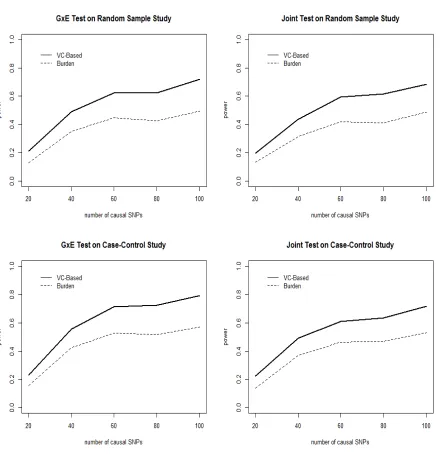
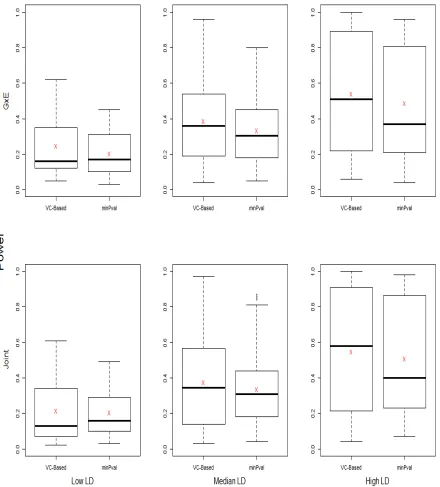
A power comparison was performed to compare the power of the proposed method and the minimum p-value method. Each two of the 29 SNPs were taken turns to be the causal SNPs such that there were total 406 scenarios. Based on the empirical LD values, we categorized each LD value into one of the three LD levels. Let LD values be ordered in an increasing manner. The first 33.33% smallest LD values were defined as low-LD values which fall in the interval of [0,0.2434). The empirical LD values were defined as median-LD values if they fall into the range of [0.2434,0.2873). Values greater than 0.2873 were defined as high-LD values.

(46)

maximum values and the mean power for each LD-level. When LD is low, the median power by applying the proposed method is slightly lower than the median power by using the minimum p-value method. Other than median power, the proposed method has higher power in terms of other quantities shown in the box-plot for low-LD. It is obvious that the average power for the proposed method is higher than the average power by applying the minimum p-value method. Among the 135 scenarios with low-LD structures, 37 (27.4%) scenarios show that the proposed method has lower power but 92 (68.1%) scenarios present higher power by applying the proposed method. For median-LD values, both the median and mean of the power for the proposed method are higher than the ones by using the minimum p-value method. Among the 136 scenarios with median-LD structures, 32 (23.5%) scenarios indicate that the power by applying the proposed method is not as high as the ones by using the minimum p-value method. But 99 (72.8%) scenarios show that the proposed method is more powerful in detecting the significance. When the LD value is relatively higher, both the median power and the mean power by using the proposed method are higher. Though the proposed method has lower power under 23 (17.0%) scenarios, 111 (82.2%) scenarios show that the proposed method is more powerful. By comparing the power at different LD levels, we observed that when the LD values is lower, the power by applying both methods are lower than the power when the LD value is either in median-level or higher-level in general. This observation is reasonable because low-LD scenarios represent the cases in which the markers contain little information about the two risk loci.

(47)

method provides good power in detecting the gene effect which improves its performance in the joint test. For median-LD and high-LD scenarios, both median power and mean power by using the proposed method are higher than the ones by applying the minimum p-value method. The reason is that the more information about the causal SNPs is correlated with the other SNPs, the more powerful the proposed method is to detect its significance.

2.4

Real Data Applications

2.4.1 Real Data Analysis for CoLaus Study Data

We applied the proposed model on a sub-sample collected from the CoLaus study which is a population-based study approved by the Institutional Ethic’s Committee of the University of Lausanne, Switzerland [68]. The primary interest of the CoLaus study is to evaluate the prevalence of risk factors in cardiovascular disease. The secondary interest is to find out any genetic determinants which are associated with those risk factors in the Caucasian population. A total sample of 6,188 individuals aged from 35 to 75 were randomly selected, their genotype information was obtained by applying the Affymetrix 500K chip.

To explore the association between the available genes and smoking status in obesity which is one of the cardiovascular disease risk factors, we were interested in testing the interaction effect of the genes available in CoLaus study and smoking status. The smoking status was treated as the environmental factor in a sub-sample of the data set from the CoLaus study. Genotype information for 8 genes is available in the study, which includes the gene GPBAR1.

Because of the missing genotypes in the data set for gene GPBAR1, data from 1937 obser-vations are available for the tests where 252 are cases. Genotype information on 11 SNPs was used in the analysis where all the 11 genetic variants are rare variant with minor allele frequency being less than 1%. As mentioned in Section 2.2.2, when most alleles are rare variants, SW is suggested.

(48)

and smoking status, we performed the GxE test on this data set. In addition to the smoking status, 9 confounders were also included in the model such age, gender, alcohol drinking status, physical activity status. In this data application, these confounders were not treated as the environmental factors interacting with the gene effects. By applying the proposed method, we obtained a p-value of 4.87×10−3. It was a strong evidence to indicate that the gene variants interplay with the smoking status in affecting obesity. By using the counting based burden test, a p-value of 0.127 was obtained which indicated non-significance of the interaction of the gene GPBAR1 and smoking status. We observed that the p-value calculated by using the proposed method is much smaller than the one by using the competing method. This result may support the observation in the simulation on the COSI based data that the proposed method is in general more powerful in detecting the significance of GxE effect.

In addition of testing the gene-environment interaction effect, we also conducted a test to examine the gene and gene-environment effects simultaneously. The proposed method had a p-value of 6.427×10−3 and the counting based burden test had a p-value of 0.15. Similar to the result we observed in the GxE test, the proposed method indicated the significance of the joint effect. However, non-significance was concluded by using the competing method. As shown in the simulation study, the results from the real data application also show that the proposed method gains more power for COSI based data in presence of rare variants.

2.4.2 Real Data Analysis for WTCCC Study Data

(49)

the genetic modifier which is expressed as the “environmental factor” in the GxE interaction for a T2D data set from the WTCCC studies. In this data set, there are total 3368 individuals remained after the quality control procedure, among them 1913 are cases and 1455 are from the control group. The case samples were collected from various sites across the UK in purpose of allowing it to be efficiently compared to the controls. The 1455 controls included in the data set were samples from the 1958 British Birth Cohort. The genotyping was conducted by applying the Affymetrix 500K chip.

We performed the GxE test by applying the proposed method, and we obtained a p-value of 4.05×10−5. There is strong evidence showing that the gene variants interact with the Body Mass Index in affecting the disease of Type 2 Diabetes. By using the minimum p-value method, the adjusted p-value of 2.72×10−3 was obtained. We observed that the p-value calculated by using the proposed method is much smaller than the one obtained by applying the minimum p-value method though both p-values are smaller than the nominal level atα= 0.05. Even though it is not absolutely that the proposed method always have lower p-values in every scenario through the results of the simulation, it still showed that the proposed method are more powerful in detecting the significance in most cases.

Additionally, the joint test was also conducted for the application on this GWAS data set. The p-value by using the proposed method is 1.81×10−10and the adjusted p-value by applying the minimum p-value method is 1.39×10−9. Compared to the p-values testing for the GxE effect, the p-values for the joint test are smaller. It might be the reason that the gene effect in this real data set has a stronger effect on an individual’s chance to have Type 2 Diabetes. However, the gene-environment interaction effect cannot be ignored because of its significance.

2.5

Discussion

(50)

computationally feasible and efficient when conducting marker-set analyses for examining the gene-environment interaction on binary traits. By showing the connection between the gen-eralized linear mixed model and the gene-similarity regression model, the proposed approach has flexibility in inference on the test statistics, while it maintains the power gain brought by aggregating the genetic information at a similarity level. In addition, the proposed method is more robust than model-based regression approaches treating the genotype information as fixed effect, such as the counting based burden test considered as a competing method in the research work. When the mean-model is misspecified or population substructure exists in the model, the counting based burden test may lead to inflation in testing the GxE interaction [76]. Even though this situation did not occur in our simulation studies, we should take great care when applying those model-based regression methods to real data sets. Because the proposed method collapses the genotype information at a similarity level and treats the genetic effects as random effects, it is comparably stable under different assumptions.

(51)

(52)

(53)

Chapter 3

Gene-Set Association Analyses for

Quantitative Traits using Linear

Mixed Models

3.1

Introduction

(54)

gene-level association studies on a same disease [45]. For that purpose, gene set association analysis (GSAA) could be used as a complementary tool to mine either existing or new association study data sets aiming to identify more multi-genic biological structure for multi-factorial disorders.

To uncover the pathway mechanisms that modulate disease risk, gene set association ap-proaches offer great potential but encounter challenges brought by the large amount of informa-tion in the existing associainforma-tion study data sets. Different from single-gene analyses, multi-gene analyses examine associations for networks or pathways which include multiple genes with com-plicated relationship among them. It requires a lot computational capacity in calculation which may involve inverting extraordinary high-dimensional matrices in order to estimate nuisance parameters. Therefore, we need to be careful in dealing with two major challenges: (1) how to better account for the within-gene multi-marker information[53, 54]; (2) how to appropriately assess association at both gene set level and gene level [61, 53]. To address the challenge of incorporating the genetic information within each gene, we collapse such information at simi-larity level. For each pair of individuals, a simisimi-larity score which measures the genetic distance between the two individuals within a gene is calculated. Thus, a large similarity matrix with

N×N dimension is computed for each gene whereN is the sample size number. In order to re-duce the dimensions of the similarity matrices, we consider the eigen-decomposition technique. To handle the challenge of assessing the associations, a variable selection technique is incorpo-rated to the variable selection on gene-specific variance components to identify significant genes from a gene set.

(55)

as-sume there is no gene-gene interactions present in the proposed model in order to investigate the underlying impact of gene sets under the additive models.

3.2

Material and Method

3.2.1 Linear Mixed Model for Gene-set Association Analysis

To demonstrate the proposed method, the following notations are defined. Suppose there are

N individuals in the study. Let Y = (Y1, . . . , YN)T be the response vector of the observed phenotypes. Specifically, quantitative traits are of interest in this project. Let X be the design matrix where each row includes the intercept and covariates for each individual. Let γ be the coefficient vector for the intercept and covariates. We assume there are K genes in the gene set, and genetic information is available for multiple markers within each gene. Let Mk be the number of loci for gene k. Let Sk be the similarity matrix where each element calculates the genetic similarity forkth gene between two individuals. Because most alleles are rare variants, we considered the weighted similarity matrix S_kW which incorporates minor allele frequencies for markers within thekth gene. Among various choices of the weights, we define the weighted similarity element forkth gene asSW

kij =

PMk

m=1wmIBS(gim, gmj )/

PM

m=1wmwith weightswm= (1−qm)24 form= 1, . . . , Mk and qm is the minor allele frequency for locus m on thekth gene [20].

Therefore, the proposed linear mixed model for quantitative traits is represented as

Y =Xγ+G1+· · ·+GK+ε, (3.1)

whereGk∼N(0, φkSkW) for k= 1, . . . , K and ε∼N(0, σIN).

(56)

Y =Xγ+Z1b1+· · ·+ZKbK+ε, (3.2)

where Zk is a N ×rk matrix such that ZkZ_kT = S_kW for k = 1, . . . , K and rk is the rank of SW

k , bk ∼ N(0, φkIrk). To identify significant genes from the gene set, a variable selection technique is considered to eliminate genes with nonsignificant associations with the disease risk; or equivalently, genes with φk’s being zero. In this work, the adaptive LASSO is applied to handle the sparseness onφk’s fork= 1, . . . , K due to its optimal properties.

3.2.2 Connection with a corresponding Gene-Trait Similarity Regression Model

Motivated by the previous work where the variance component model has been shown its connections to a gene-trait similarity regression model when markers from one gene is of interest [21], we prove the variable selection on the variance components in Equation (3.1) is equivalent to select the gene-specific coefficients for the gene-trait similarity regression model in Model (3.3). Let Tij be the trait similarity between individuals i and j which is defined as Tij = (Yi−µ0i)(Yj −µ0j) where the conditional mean µ0i = Xiγ [21, 22]. Similar to the association analysis for marker-set on a single gene, the corresponding gene-trait similarity regression model for gene set association analysis is

E(Tij|X, S) =a1×S1ij +a2×S2ij +· · ·+aK×SKij, (3.3)

where Skij is the similarity matrix for the gene k and the weighted similarity matrix SkijW is considered in this work.