A Memory Hierarchy- and Network Topology-Aware Framework for Runtime Data Sharing at Scale.

(1)

ABSTRACT

ZHANG, WENZHAO. A Memory Hierarchy- and Network Topology-Aware Framework for Runtime Data Sharing at Scale. (Under the direction of Dr. Nagiza F. Samatova.)

Data analytics is often performed in a post-processing manner, as the data generated by an application is first written to the file system, for example parallel file system (PFS), and then read out to dynamic-random-access-memory (DRAM) for analytics, requiring substantial I/O time. Runtime data sharing across multiple applications is a promising alternative approach towards avoiding the increasing I/O bottlenecks. For instance, the data generated by a running application can be moved to a DRAM-based server staging space, where that data is then retrieved by various client analytics applications, such as visualization and transformation. Thus, data generation and analytics can run concurrently, and slow PFS access is replaced by fast DRAM access.

In this dissertation, we illustrate the value of the proposed framework using large scale scientific datasets generated and shared over modern supercomputers. Specifically, we demon-strate that our framework enables the runtime sharing of the Adaptive Mesh Refinement (AMR) scientific data, unlike traditional uniform mesh data. AMR represents a significant advance for large-scale scientific simulations. By dynamically refining resolutions over time and space, AMR simulations generate hierarchical, multi-resolution, and non-uniform meshes. This kind of refinement provides sufficient precision for regions of interest at finer levels while avoiding unnecessary data generation for regions of non-interest. However, due to unable to handle the dynamic characteristics of AMR data and the dynamic runtime behaviors of AMR simulations, existing methods are not applicable to support runtime AMR data sharing for scientific analytics. In this dissertation, we propose a framework to facilitate runtime AMR data sharing for scientific applications, with the goals of realizing effective AMR data access and further optimizing data access performance over the staging space by exploring memory hierarchy and network topology of modern supercomputers. We first present a purely DRAM-based framework to support runtime AMR data sharing. By employing an architecture with dedicated server processes for metadata management, an efficient and balanced AMR data distribution policy and a poly-tree-based spatial index, the framework enables client applications to effective write/retrieve AMR data to/from the staging space.

(2)

distribution across network topology.

(3)

A Memory Hierarchy- and Network Topology-Aware Framework for Runtime Data Sharing at Scale

by Wenzhao Zhang

A dissertation submitted to the Graduate Faculty of North Carolina State University

in partial fulfillment of the requirements for the Degree of

Doctor of Philosophy

Computer Science

Raleigh, North Carolina

APPROVED BY:

Dr. Rada Y. Chirkova Dr. Kemafor Anyanwu Ogan

Dr. Ranga Raju Vatsavai Dr. Nagiza F. Samatova

(4)

BIOGRAPHY

(5)

ACKNOWLEDGEMENTS

First and foremost, I am very grateful to my advisor, Dr. Nagiza Samatova. I definitely could not have reached this point without her consistent guidance and support in the past four and a half years. I am very thankful to my committee members, Dr. Rada Chirkova, Dr. Kemafor Ogan, and Dr. Raju Vatsavai, for taking their valuable time to serve on my thesis committee, and for offering their insights in this dissertation.

This dissertation would not have been completed without the help from Dr. Samatova’s research group. I am very grateful to Xiaocheng Zou and Houjun Tang for their priceless help for my PhD research. Additionally, I would like to thank Steve Harenberg and Stephen Ranshous for their help with my research paper writing.

I have had the honour of collaborating with researchers at national laboratories: Drs. Suren Byna, Kesheng (John) Wu, Bin Dong, Dan Martin, Hans Johansen, and Dharshi Devendran from Lawrence Berkeley National Laboratory, and Scott Klasky, Qing (Gary) Liu from Oak Ridge National Laboratory.

(6)

BIBLIOGRAPHY . . . . 53

78

(8)

LIST OF TABLES

Table 4.1 Variables for the algorithm of read memory hierarchy resource . . . 60

Table 4.2 RID index size for each simulation’s dataset . . . 66

Table 4.3 Values for key system-specific parameters in the coarse model . . . 71

(9)

LIST OF FIGURES

Figure 2.1 The visualization graph of a 1GB block-structured AMR dataset generated by BISICLES [20]. The coarsest (or lowest) level (level 0) covers the entire global data domain. A finer (or higher) level is generated by refining a set of boxes on the adjacent coarser level, only covering some subregions of interest with higher resolution as defined by a refinement ratio. The boxes at the finer levels represent spatial regions of more interest. . . 10 Figure 2.2 A uniformly partitioned virtual bounding box over the finest level of the

AMR data in Figure 2.1. These partitions would be distributed to the staging space according to a space-filling curve (e.g., Hilbert), leading to an unbalanced workload distribution, among other issues. . . 11 Figure 2.3 The client-server architecture of AMRZone consists of two types of server

processes: (1) mservers that only manage metadata, recording how AMR boxes are distributed across dservers and constructing a spatial index; and (2)dservers that only manage the binary data. Note that Application1 and Application2could be simulations or other data analytics programs. Also note that AMRzone does not limit the number of applications that can connect to the server side. . . 12 Figure 2.4 A spatial query over AMR data. Typically, boxes are retrieved in multiple

levels, rather than a single level. The boxes at level 1 are refined from bigger boxes at level 0. . . 16 Figure 2.5 The polytree-based spatial index for AMR data. Tree nodes correspond to

AMR boxes. Directed edges denote refinement relationship. It effectively represents the many-to-many refinement relationships of AMR boxes across different levels. . . 17 Figure 2.6 Configuration details for the scalability comparison experiments. The

row header denotes four domain sizes and the column header gives four partition sizes. The format,$B$C($N) /$S($N), denotes the total number of boxes(B), the total number of parallel client processes(C), the total number of client nodes(N), the total number of DataSpaces server or AMRZone dserver processes(S) and the total number of server nodes(N). 21 Figure 2.7 Results of weak scalability comparison experiments between AMRZone

(10)

Figure 2.8 Configuration details for two sets of AMRZone experiments, one over expanded BISICLES AMR datasets, one over synthetic uniform datasets. Row 2, 6 give the dataset size(GB) for one time-step. For the synthetic datasets, it also gives global dimension size. Row 3, 7 give the total number of client processes(C), the total number of client nodes(N), the total number of dserver processes(S) and the total number of server nodes(N) for the corresponding time-step. Row 4, 8 give the total number of boxes(B) and box sizes(MB) in the corresponding time-step. For the synthetic datasets, it also gives the dimension size for a box. In row 2 and 4, the values for BISICLES datasets are average ones. . . 23 Figure 2.9 Results of boxes write/read performance testing for AMRZone over real

AMR datasets, with comparisons on synthetic uniform data, totally 10 time-steps. In the worst case, AMR data related task demands more than 36% additional execution time, in the best case it is 2% more. In 5 cases (out of 8), AMR data coupled write/read needs less than 10% more time. Note these are not weak scaling testings. . . 24 Figure 2.10 The statistics for the AMR data workload on dserver processes. The row

header denotes the four domain sizes and total number of dserver processes respectively. The column header denotes the minimum, maximum, average, median, first quartile and third quartile for the workload on dservers for an experiment related to each domain size. Note, for each domain size, there are 10 time-steps of AMR data written to the server space. . . 24 Figure 2.11 Configuration details for two sets of AMRZone experiments over expanded

BISICLES datasets, one for spatial constrained data retrieval, one for AMR boxes retrieval. Row 2, 6 give the amount data(GB) retrieved for a time-step. Row 3, 7 give the total number of client processes(C), the total number of client nodes(N), the total number of dserver processes(S) and the total number of server nodes(N) for the corresponding time-step. Row 4, 8 give generally the total number of boxes(Boxes) and box sizes(MB) in the retrieved data for a time-step. The values in row 2, 4, 6 and 8 are average ones. . . 26 Figure 2.12 Results of spatially constrained data retrieval performance testing for

AMRZone over AMR datasests, with comparisons of AMR boxes read, totally 10 time-steps. Note these are not weak scaling testings. . . 27

Figure 3.1 The visualization graph of a 1GB block-structured AMR dataset generated by BISICLES [20]. BISICLES is a large scale simulation for modeling Antarctic ice-sheets. . . 33 Figure 3.2 The polytree-based spatial index for AMR data in AMRZone. Tree nodes

(11)

Figure 3.3 The illustration of 2D AMR data coupled spatial access patterns detection for a client process. The accessed region over time-step n is compared with the one over time-step n-1. After finding the boundary variation (the right boundary moves one unit toward the right), the framework predicts this change will continue, and it generates a new predicted spatial access region by applying the same trend. This new predicted region is used for prefetching data of time-step n+1. . . 37 Figure 3.4 The timing sequence diagram for prefetching, involving a client process, an

mserver process’s thread, a dserver processs and the dserver’s dedicated prefetching thread. For a dserver, there is a time period between retrieving a time-step’s data and receiving the data request of the next time-step, which can be leveraged to do prefetching for the next time-step. . . 38 Figure 3.5 Illustration of how redundant messages can be sent during prefetching. At

level 0, the two spatial regions overlap with box0 1 and box0 2, respectively, and prefetching messages are sent for those two boxes. However, at level 1, box1 2 overlaps with both box0 1 and box0 2, so multiple messages are sent for box1 2. . . 39 Figure 3.6 The throughput difference between nodes of different topology distance

on Cori [19] (the testbed for this work). For details of how the topology distances are calculated, please refer to Section 3.3.4. The result is based on a micro benchmark, which sends 1 MB ping-pong messages between a pair of nodes, repeating the process 30,000 times. This benchmark setup (small message size and big number of messages) resembles AMR data, as each AMR box is usually not very large (from a few KBs to a dozen MBs), but the number of boxes in a time-step is high (from several thousands to tens of thousands). At any given time, only one pair of nodes are communicating with each other. Average experiment values are reported. 40 Figure 3.7 An illustration of the runtime factors that our framework must consider

when determining where to place an AMR box. The mserver must not only consider topology distance, but also the size of each AMR box, and the workload of all staging nodes which keep changing at runtime. For example, in the figure, in terms of topology distance node 0 should be chosen to place the incoming box, but in terms of workload, node 3 should be selected. The final choice should be appropriately balanced among all factors. . . 41 Figure 3.8 The effectiveness of our framework handling the condition when the staging

space is becoming full, with comparison of direct SSDs and PFS access (not involving our framework’s staging space). Compared to directly writing data to SSDs, with added time periods to imitate computation periods, our framework can achieve average 72.85% and median 71.93% improvement respectively. . . 46 Figure 3.9 Illustration of the 11 major Antarctic ice shelves. The spatial regions of

(12)

Figure 3.10 The effectiveness of our framework performing prefetching for spatially constrained access, compared to direct SSDs and PFS access (not involving our framework’s staging space). The spatial access patterns of client processes are based on the 11 major Antarctic ice shelves on a BISICLES dataset, as illustrated in Figure 3.9. Each client accesses one such region. For our framework with patterns detection and prefetching, the average and median performance improvement are 26.47% and 26.03% respectively. 49 Figure 3.11 On Cori, the effectiveness of our framework’s topology-aware runtime

AMR data placement optimization, compared to direct SSDs and PFS access (not involving our framework’s staging space). For writing, the average and median improvements of topology-aware optimization are 18.08% and 18.73%, respectively. For reading, the average and median improvements are 10.57% and 10.49%, respectively. . . 50 Figure 3.12 On Titan, the effectiveness of our framework’s topology-aware runtime

AMR data placement optimization, compared to direct PFS access (not involving our framework’s staging space). Titan does not have SSDs, so no comparison to direct SSDs access is possible. Note that all data in a time-step is used, and no spatial access patterns involved. For writing, the average and median improvements are 24.85% and 26.39%, respectively. For reading, the average and median improvements are 17.21% and 16.43%, respectively. . . 51

Figure 4.1 SSDs and advanced PFS write performance comparison using one Sith compute node at Oak Ridge National Lab. SSDs’ write performance is worse than advanced PFS. Data written size in each test is 1GB. Refer to Sec. 4.4.1 for details of the Sith cluster and PFS striping policy. . . 55 Figure 4.2 Framework architecure overview: the gray components are our

contribu-tions and could be categorized as online and offline modules. The online modules have two major functionalities, executing a read algorithm and data management. They rein over all online read and write flows through all memory layers. . . 56 Figure 4.3 Scenario where read specially arranged PFS cache could relieve contention

on the SSD: the first process on each node reads the PFS cache which is specially distributed across OSTs in disjoint manner. Because of reduced parallel read contention on the SSD, no contention between the processes that read the PFS, and PFS’s high sequential read speed, the actual performance could be improved. . . 58 Figure 4.4 Algorithm for read memory hierarchy resource. Applying a two-step coarse

(13)

Figure 4.5 State flowing chart for managing aggregated write buffers to interleave write and read operations to hide data write overhead on file systems. . . 62 Figure 4.6 Every process accesses all OSTs or a subset of OSTs. Contention is severe

in this case. . . 62 Figure 4.7 Two ideal cases that read contention on OST is minimized. Case1 process

number smaller than OST’s; Case2, process number bigger than OST’s. . 62 Figure 4.8 MLOC’s VC-SC storage layout. Dataset is first binned to treat

value-constrained access(VC) as first priority, each bin is partitioned by Hilbert Curve order for spatial constrained access(SC) as second priority. RID denotes the index for a value if the dataset is linearized in row-major order 66 Figure 4.9 Three types of domain decomposition as benchmark used in spatial

con-stained(SC) access evaluation. . . 67 Figure 4.10 Evaluation for spatial constained(SC) access, access 10% and 20% region

using three types of domain decomposition. Performance on VC-SC layout is worse than the unoptimized dataset because SC is treated with minor priority, thus SC access suffers more overhead. This is the compromise the layout must pay in order to avoid generating multiple full copies of datasets, please refer to 4.4.2 for details. . . 68 Figure 4.11 Evaluation for value constained(VC) access, 10% and 20% data selectivity

using region-value and region-only access. . . 70 Figure 4.12 10% and 20% spatial constained access(SC) on SSD cache: the U-shape

lines show that increasing the number of processes cannot always reduce access time, which is caused by read contention on SSDs’ file system. . . . 71 Figure 4.13 Improvement for 10% and 20% spatial constained(SC) access by SSD-PFS

hybrid read: applying one or two processes per node to read carefully arranged PFS cache that is distributed across disjoint OSTs, contention on the SSD could be effectively relieved. Please refer to Fig. 4.3 for the illustration of the read strategy. . . 72 Figure 4.14 Model correctness evaluation. When 100%, 90%, 80% and 70% PFS cache

available, the prediction is generally valid. For 60% case, the prediction is invalid. Overall precision is about 90%. . . 74 Figure 4.15 Write SSD methods evaluation: write data which is read through 10% and

(14)

CHAPTER

1

INTRODUCTION

Post-processing-based data analytics typically involves writing the generated data first to parallel file system (PFS), then reading the data out from PFS to dynamic-random-access-memory (DRAM) for analytics. As hard drivers based PFS is orders of magnitude slower than DRAM [10, 37, 54, 65], this approach experiences substantial I/O time. Runtime data sharing is an effective approach for avoiding the high I/O latency incurred by post-processing methods [26, 69]. The principle idea of runtime data sharing is to assemble a DRAM-based server staging space on a set of dedicated compute nodes. Client processes, which run over another set of nodes, can be simulations, producing data and writing to the staging space, or analytical applications, reading data from the staging space [5, 27]. Thus, data generation and analytics can be executed concurrently, and slow PFS access is replaced by fast DRAM access.

(15)

memory and storage, while retain or even improve computation accuracy [16, 47]. Many scientific applications have successfully adopted the AMR model, such as BISICLES [20] (a large scale Antarctic ice-sheet modeling program), Enzo [18, 51] (a astrophysics simulation for cosmological structure formation analytics), and GenASiS [9, 12, 31, 32] (a simulation for studying neutron star mergers and core-collapse supernovae). In this dissertation, we focus on block-structured AMR, which consists of a collection of disjoint rectangular boxes (or regions) at each refinement level [76].

However, the great flexibility of AMR is also its Achilles’ heel. Specifically, a set of dynamic characteristics are inherent to AMR data, namely, the numbers, sizes, and locations of the AMR boxes, are usually unpredictable before a simulation run and keep changing as the simulation progresses [69]. Moreover, AMR simulations demonstrate several dynamic runtime behaviors, namely largely and heterogeneously changing resource requirements (DRAM, CPU, and network bandwidth) [44]. Due to incapability of adapting to those characteristics, existing methods cannot facilitate runtime AMR data sharing across scientific applications. Moreover, flattening and unifying AMR boxes to make the data compatible with existing methods is not a viable solution as AMR’s advantages would be lost and significant overhead would be introduced [76].

Therefore, we present a framework to facilitate runtime AMR data sharing across scientific applications. First, we present a purely DRAM-based framework to support efficient runtime AMR data sharing, which has dedicated server processes for handling metadata, balanced AMR data placement policy and a poly-tree-based [21] spatial index to address the issues introduced by the dynamic characteristics of AMR data.

Based on this, we further present a set of methods to extend the framework. The upgraded framework is able to store data over Solid State Drives (SSDs) when the DRAM space is full, and optimize AMR data access performace over the staging space by detecting common spatial AMR data retrieval patterns and adaptively distributing AMR data across network topology.

We finally present a set of approaches to address some key performance issues plaguing SSDs, such as read contention and files fragmentation. In the following subsections, we briefly summarize the challenges and contributions for our work.

1.1

A DRAM-Based Framework for Runtime

AMR Data Sharing

1.1.1 Problems and Challenges

(16)

server processes of the staging space would incur significant overhead because of the dynamic characteristics inherent to AMR data and because the data being written to the staging space could arrive in any order.

Second, to retain high data access throughput, the framework should have a balanced workload distribution at runtime for the nodes on the server side. However, static data domain partitioning and distribution methods (e.g., space-filling curves [55]) typically fail to achieve this goal for AMR data. Due to the dynamic characteristics of AMR data, those methods can not determine a suitable partition size until most of the AMR boxes of a domain have been received and examined, which would produce a large runtime overhead.

Third, to support data retrieval of specific spatial regions, the framework needs an efficient online spatial index that can satisfy AMR’s unique spatial data access patterns, which typically involve accessing multiple boxes across multiple levels [76]. However, existing spatial indices do not effectively catch the hierarchical and non-uniform structure of AMR data.

1.1.2 Approach and Results

To the best of our knowledge, runtime AMR data sharing across scientific applications has not been well explored. In order to address the architecture issue, the proposed framework has dedicated server processes to handle only metadata, such as tracking the placement of each AMR box and building a spatial index over the metadata. It also has server processes which are only responsible for binary data, namely binary data storage and transmission. With this design, the framework is able to significantly reduce AMR metadata synchronization overhead.

In order to achieve overall balanced AMR data distribution over the staging space, the metadata server processes of the framework do not perform any static data domain partition, thus do not require any static global domain information before a simulation run. Instead, the metadata servers check each received AMR box and determine its placement at runtime. To support this task, an metadata server maintains a collection of workload tables to monitor how much data is stored on each binary data server and each compute node.

In order to facilitate efficient spatially constrained AMR data retrieval, the framework constructs a poly-tree-based [21] spatial index over the metadata. This spatial index can represent the multi-level and many-to-many AMR boxes relationships well, and support efficient spatial AMR data retrieval.

(17)

1.2

Exploring Memory Hierarchy and Network Topology for

Runtime AMR Data Sharing

Our previous approach addresses how to achieve efficient runtime AMR data sharing in a purely DRAM-based staging space. However, the purely DRAM-based method is becoming insufficient, as the volume of data being generated by scientific applications continues to grow, often exceeding the capacity of DRAM by 100% or more [43], necessitating the use of the PFS, thus increasing access latency. To address this capacity issue, solid state drives (SSDs) have been utilized as an overflow space for when DRAM fills [43]. SSDs are chosen as they are usually two orders of magnitude faster than hard disk drives, which the PFS uses, and provide more than ten times the capacity of DRAM [37].

To develop such a memory hierarchy-aware runtime AMR data sharing framework, three major challenges must be addressed. First, to avoid out-of-memory (OOM) errors when receiving data from clients, the framework must know when to move data from DRAM to another part of the memory hierarchy. To predict when the DRAM space will be full, the framework would need to know the ingress throughput; however, AMR simulations’ runtime output is typically unpredictable [44], resulting in a highly dynamic throughput in the staging space. As this issue is rare in the domain of uniform mesh data, it is a challenge brought on by AMR data.

Second, because SSDs are about one order of magnitude slower than DRAM [37], being able to identify spatial read patterns to facilitate prefetching data from the SSDs into DRAM is desirable. Unfortunately, due to the multi-level, non-uniform structure of AMR data, the techniques used in [43] are scarcely applicable, requiring new methods be developed.

Third, in order to further optimize data access performance, the framework needs to distribute data across the staging space properly to reduce network transmission latency at runtime. This is not as straightforward as it would be with uniform mesh data [60], as the sizes of AMR boxes are unknown a priori and highly irregular when generated [69].

To the best of our knowledge, a framework to support runtime AMR data sharing between scientific applications that employs more than the DRAM portion of the memory hierarcy and accounts for network topology has not been proposed. By greatly extending our research of a purely DRAM-based runtime AMR data sharing framework (discussed in the previous subsection), we address the above challenges.

(18)

can monitor the changes in the throughput to retain an accurate estimate of when DRAM will reach capacity. Thus make it possible to move data to the SSDs in a timely manner.

Second, in order to adapt to the highly irregular structure of AMR data and prefetch the data from SSDs to DRAM to bridge the speed gap between the two memory layers, the framework can employ an AMR data-aware algorithm to effectively search all AMR levels to generate spatial regions for prefetching.

Third, in order to reduce the network transmission latency, the framework can utilize a multivariate cost model to adaptively distribute AMR data over the network topology. The model will be able to consider factors, such as box sizes, staging space workload balance and topology distrances at runtime.

When tested over real AMR datasets, besides effectively manage the staging space without any OOM errors, the framework’s spatial access patterns detection and prefetching methods demonstrate about 26% performance improvement, and its runtime AMR data placement optimization can improve performance by up to 18%.

1.3

Memory Hierarchy Aware Data Read Performance

Optimization

Many scentific data analytics applications are becoming I/O bound as simulations in modern high performance computing (HPC) systems, such as S3D combustion [15] and FLASH reactive hydrodynamic equations [3], are generating increasingly large datasets. Further compounding this problem, the huge volume of data continuously widens the speed and capacity gap between DRAM and hard disk drives (HDDs). To address this bottleneck, methods for optimizing read performance have been proposed in two independent parallel lines of researches: memory hierarchy exploitation and storage layout reorganization.

Regarding the first line, although the related methods achieve their goal by employing SSDs in a pivotal role combined with either PFS or DRAM, they still lack some considerations that we argue to be important. First, read contention on SSDs may cause up to 50% performance reduction, greatly compromising the effectiveness of the devices. Second, attention to supporting methods are required to maintain a near optimal operating environment for SSDs, namely to handle high write latency and fragmentation issues on the devices.

(19)

several methods to optimize different categories of patterns, but in this case it is necessary to keep more than one full copy of dataset, which is not storage efficient.

In order to relieve the reading contention issue of SSDs, we propose a general purpose memory hierarchy aware online read algorithm. It could detect possible read contention on SSDs and utilize memory hierarchy resouce to mitigate the issue. In order to maintain a near optimal operating environment for SSDs, we also present a set of data management methods. They are able to orchestrate data across different memory layers to handle issues that may compromise the effectiveness of SSDs, such as fragmentation.

Note that, those methods only work for the cases that each individual SSD device is explicitly available for access, for example SSDs are installed on each compute node, so that the proposed methods can explicitly manage data access behaviors and data organization on the SSDs. Otherwise, if SSDs are installed on a set of dedicated I/O nodes, and only an abstract access interface is provided, such as the case of Cori [19], those proposed methods are unapplicable.

In order to optimize common access patterns without creating multiple full copies of datasets, we present methods to cache carefully selected data chunks onto SSDs. The methods can facilitate both spatial constrained and value constrained data read access.

(20)

CHAPTER

2

A DRAM-BASED FRAMEWORK FOR

RUNTIME AMR DATA SHARING

2.1

Introduction

Scientific data analytics are often performed in a post-processing manner, as the data generated by a simulation is first written to the file system and then read for analytics, requiring substantial I/O time. Runtime data sharing across multiple applications is a promising alternative approach towards avoiding these increasingly severe I/O bottlenecks [73]. For instance, the data generated by a running simulation can be moved to the memory of a set of dedicated compute nodes where that data is then retrieved by various analytics applications, such as visualization and transformation [5, 27].

To facilitate this runtime data sharing, related methods typically organize a set of nodes to provide an in-memory data staging and management space on the server side. Through client side APIs, applications running on other nodes can efficiently write data to the space and retrieve data from it. Although these methods are effective at handling uniform mesh data, they currently do not support adaptive mesh refinement (AMR) data.

(21)

for regions of interest at finer levels while avoiding unnecessary data generation for regions of non-interest [76]. In this work, we focus on block-structuredAMR, which consists of a collection of disjoint rectangular boxes (or regions) at each refinement level [76].

To the best of our knowledge, runtime AMR data sharing across applications has not been well explored. This is a non-trivial task due to the dynamic characteristics inherent to AMR data; namely, the numbers, sizes, and locations of the AMR boxes, are usually unpredictable before a simulation run and keep changing as the simulation progresses. These characteristics prevent existing methods from effectively handling AMR data. Moreover, flattening and unifying AMR boxes to make the data compatible with existing methods is not a viable solution as AMR’s advantages would be lost and significant overhead would be introduced [76].

To create a framework that facilitates runtime AMR data sharing across multiple applications, there are three major challenges that should be addressed. First, the architecture of such a framework should enable efficient online AMR data management. However, runtime AMR metadata synchronization across distributed server processes would incur significant overhead because of the dynamic characteristics inherent to AMR data and because the data being written to the staging space could arrive in any order.

Second, to retain high throughput, the framework should have a balanced workload distri-bution at runtime for the nodes on the server side. However, static data domain partitioning and distribution methods (e.g., space-filling curves [55]) typically fail to achieve this goal for AMR data. Due to the dynamic characteristics of AMR data, those methods can not determine a suitable partition size until most of the AMR boxes of a domain have been received and examined, which would produce a large runtime overhead.

Third, to support data retrieval of a specific spatial region, the framework needs an efficient online spatial index that can satisfy AMR’s unique spatial data access patterns, which typically involve accessing multiple boxes across multiple levels [76]. However, existing spatial indices do not effectively catch the hierarchical and non-uniform structure of AMR data. Moreover, due to the dynamic nature of AMR, how to build the spatial index efficiently at runtime while maintaining high data transmission performance poses another challenge.

In this work, we propose AMRZone, a framework for facilitating runtime AMR data sharing across multiple scientific applications. In addition to addressing the above challenges, AMRZone even demonstrates comparable performance and scalability with existing state-of-the-art work when tested over uniform mesh data; in the best case, our framework achieves a 46% performance improvement. Specifically, towards addressing the above challenges, we make the following contributions through our framework:

(22)

Online balanced AMR data distribution on the server side, by adopting a runtime workload policy based on AMR boxes (Section 2.3.2).

A polytree-based online spatial index to facilitate spatially constrained AMR data retrieval (Section 2.3.3).

2.2

Background

DataSpaces [25] is the current state-of-the-art framework for runtime data sharing across multiple scientific applications over uniform mesh data. In the following sections, we explain three major issues that prevent it from effectively supporting AMR data. Although other frameworks (described in Section 2.5) can provide a distributed and in-memory data manipulating space, we select DataSpaces for comparison because it is the only framework that can build an explicit online index over the distributedly staged data as well as provide effective data access APIs, both of which are key features that facilitate runtime data sharing across applications.

At the heart of DataSpaces is a distributed hash index that enables efficient data retrieval from spatial regions of interest. The index is based on a Hilbert space-filling curve [50] that is used to partition a global data domain into subregions (or partitions) and then distribute these partitions evenly to the staging nodes. Although effective at handling uniform mesh data, there are several non-trivial issues that would arise if DataSpaces were applied to AMR data. A 1GB 5-level dataset generated by BISICLES(a large-scale Antarctic ice sheet modeling code for climate simulation) [20] is used to illustrate the hierarchical and non-uniform structure of AMR data. Its visualization is shown in Figure 2.1.

2.2.1 Issue I: Architecture

DataSpaces has a client-server architecture. The server side is composed of a set of server processes (or servers) running on different nodes to form a virtual in-memory space. The client side is a collection of APIs used to interact with the space. Each server process is responsible for both maintaining metadata (the distribution of data subregions) and transporting data. The server side demands a pre-defined global domain size before any data is written or read. Therefore, once a partition size is determined, it is easy to know the total number of subregions and how to map each one to the servers evenly, before any client connects to the servers. If a client needs to access a certain region of data, it can get the metadata by contacting any server, making the metadata management of this architecture very effective over uniform mesh data.

(23)

Figure 2.1 The visualization graph of a 1GB block-structured AMR dataset generated by BISI-CLES [20]. The coarsest (or lowest) level (level 0) covers the entire global data domain. A finer (or higher) level is generated by refining a set of boxes on the adjacent coarser level, only covering some subregions of interest with higher resolution as defined by a refinement ratio. The boxes at the finer levels represent spatial regions of more interest.

distribution before a simulation run (see Section 2.2.2 for details). Thus, in order to maintain consistent metadata between all the servers to monitor the overall workload status, it is necessary to frequently exchange metadata between all servers at runtime. This frequent communication between the servers results in a high runtime synchronization overhead.

2.2.2 Issue II: Online Data Organization

(24)

Figure 2.2 A uniformly partitioned virtual bounding box over the finest level of the AMR data in Figure 2.1. These partitions would be distributed to the staging space according to a space-filling curve (e.g., Hilbert), leading to an unbalanced workload distribution, among other issues.

and distributed to the server nodes, it would be too time consuming to dynamically optimize an unbalanced workload distribution, as that would require retrieving, repartitioning, and redistributing all of the staged data. On the other hand, attempting to achieve a balanced workload distribution at runtime would be costly because the majority of the AMR boxes must be received and evaluated first before a suitable partition size can be determined. Arguably, any partition methods that are based on space-filling curves (e.g., Z, Peano, Hilbert curves, etc. [55]) would not be effective at evenly distributing AMR data onto a set of nodes at runtime.

(25)

Application1

… ……… Client API

Node0 mserver Process

Thread Pool

… T1 T2 T3 TN Node1

……

dserver Process1 dserver Process2

dserver ProcessN

Metadata Flow

Binary Data Flow

NodeN

……

dserver Process1 dserver Process2

dserver ProcessN Proc1 Proc2 ProcN

… ………

Application2 Client API Proc1 Proc2 ProcN

Figure 2.3 The client-server architecture of AMRZone consists of two types of server processes: (1) mserversthat only manage metadata, recording how AMR boxes are distributed across dservers and constructing a spatial index; and (2)dserversthat only manage the binary data. Note that Application1andApplication2could be simulations or other data analytics programs. Also note that AMRzone does not limit the number of applications that can connect to the server side.

2.2.3 Issue III: Online Spatial Index

Analytics over AMR data are usually performed over the boxes from all levels that overlap with the specified spatial region [76], rather than just the boxes on a single level, as illustrated in Figure 2.4. However, to retrieve AMR boxes from all levels using Datapsace’s hash index, where partitions are given by the Hilbert space-filling curve, it would be necessary to check the boxes in every partition that overlaps with the specified query region. This kind of linear checking is inefficient when faced with a large number of parallel queries. Moreover, it would appropriate CPU resources that could otherwise be used for processing other runtime tasks (e.g., data transportation), reducing parallelism.

2.3

Methods

(26)

2.3.1 Architecture

AMRZone consists of a distributed client-server architecture. The server side consists of a set of server processes (or servers), which run on a user-defined collection of compute nodes, providing a shared memory-based virtual data staging and management space with public data access functions. The client side is a set of APIs that can be integrated by running applications (e.g., simulations or other data analytics programs) to access (e.g., write, retrieve, or update) the data in the space. The architecture of ARMZone is depicted in Figure 2.3.

As described in Section 2.2.1, the architecture design in which a server process is responsible for both maintaining metadata and transportating data introduces a significant performance overhead with AMR metadata management. To avoid this issue, AMRzone uses servers that exclusively handle either the metadata task or the data transportation task:

Mservers - responsible for metadata, namely recording on which data-server an AMR box is placed and building a spatial index

Dservers - manage the actual binary data of AMR boxes, such as data storage and transmission

The mservers act as coordinators between the clients and dservers. For example, when an application demands to write or read a certain region of data, it first contacts an mserver. The mserver updates or searches the metadata, and sends back the communication addresses of a certain set of dservers where the application can establish connections and perform the data transportation. Note that our framework does not limit the number of applications that connect to the data staging space.

With this architecture design, AMRzone is able to significantly reduce metadata synchro-nization. To accomplish this, AMRZone uses a single mserver to handle all metadata associated with a single time-step of a simulation. This design eliminates the need to exchange metadata at runtime for the servers, preventing a significant performance overhead.

(27)

able to achieve a high parallelism. In fact, as we show in Section 2.4.1, this architecture gives satisfactory performance when facing more than 10,000 writers/readers in parallel.

The write and read functions associated with the client APIs use AMR boxes as the atomic units. We make this design decision because AMR data is typically accessed by boxes. For example, in Chombo [17], a popular block-structured AMR data manipulation framework, a level’s domain is represented by a collection of boxes. In a previous AMR data analytics method [76], analysis tasks are performed over a set of boxes. For more details of the initial prototype implementation of the framework, refer to Section 2.3.4.

2.3.2 Online Data Organization

As stated in Section 2.2.2, when space-filling curves are used to partition and distribute AMR data, it is difficult to avoid an unbalanced online workload placement at the staging space. To address this issue, the mservers of AMRzone do not perform a static partition of the data domain and, thus, do not require any global domain information. An mserver checks each received AMR box and determines its placement at runtime. To support this task, an mserver maintains a collection of workload tables to monitor how much data is stored on each dserver and each node.

Algorithm 2.1 gives the general procedure that the mservers use to decide on which dserver to place the binary data of an AMR box after a write-AMR-box request is received. First, it searches the dserver nodes workload table for a node with minimum workload (lines 1-7). Next, it finds the dserver process with the minimum workload on the specified node (line 9-14). By considering each of the AMR boxes received at runtime, the algorithm avoids any static and uniform data domain partition, thus realizing a far better data distribution balance across the staging space than space-filling curves. According to the results in Section 2.4.2, our framework’s read performance over AMR data is comparable to the read performance over balanced uniform mesh data, demonstrating the effectiveness of this workload assignment policy.

To store the metadata for an individual AMR box, we employ a linear hash table because of its effective insertion and lookup operations. A cell of a hash table corresponds to an AMR box and a combination of a box’s coordinates is used as the hash key. Inside each dserver process, there is also a collection of hash tables corresponding to all the levels of all time-steps. These are used to store and retrieve the boxes’ binary data. When a dserver receives the binary data of a box, it only needs to insert the box to a hash table.

(28)

Algorithm 2.1: Algorithm of an mserver determines the placement for an AMR box at the staging space

Input: 1D array of the workload for all staging nodes: T1[]; the size of T1: N.

Input: 2D array of the workload for all dservers for each staging node: T2[N][]; the size of T2[N]: S[]

Result: A suitable dserver to place the box:ds index

1 /*Find the node with minimum workload:*/

2 max wl =maximum possible workload f or a node 3 node index= 0

4 for i={0, ..., N−1}do 5 if T1[i]< max wlthen 6 max wl=T1[i] 7 node index=i

8 /*Find the dserver process with minimum workload:*/ 9 max wl =maximum possible workload f or a dserver 10 ds index= 0

11 for i={0, ..., S[node index]−1}do 12 if T2[node index][i]< max wl then 13 max wl=T2[node index][i] 14 ds index=i

2.3.3 Online Spatial Index

To facilitate AMR data sharing across multiple applications, the framework needs to be able to effectively retrieve data from a specific spatial region of interest. As shown in a previous AMR data analytics work [76], spatial queries over AMR data usually request data from all levels, rather than a single level (as illustrated in Figure 2.4). To achieve this goal, an mserver’s linear hash table, which is used to store the metadata of the AMR boxes (as described in 2.3.2), is far from efficient. The hash table requires linearly checking all AMR boxes, reducing parallelism by competing with CPU resources from other runtime tasks, such as data transportation.

(29)

Level0

Level1

Level0

Spatial

Region

Figure 2.4 A spatial query over AMR data. Typically, boxes are retrieved in multiple levels, rather than a single level. The boxes at level 1 are refined from bigger boxes at level 0.

number of boxes and add more complicated runtime procedures to the framework. Not only could this compromise index construction and search performance, but it could also introduce network overhead due to more boxes write/read operations.

To overcome those issues, we propose a polytree [21] based spatial index for AMR data, as shown in Figure 2.5. The root of the polytree represents a single time-step of the simulation. Each level of the tree corresponds to an AMR level, and the nodes at the same level of the tree represent the AMR boxes of that level. Finally, the directed edges from coarser level nodes to finer level nodes represent refinement relationships. This polytree index is constructed over the boxes’ metadata inside the mservers.

Given this index structure, the many-to-many AMR boxes’ refinement relationships are well represented and spatial queries can be answered efficiently. After finding the AMR boxes at a level that overlaps with a given spatial region, the searching at the next finer level can be limited to the boxes which are refined from those found boxes at the coarser level. By performing a search in this manner, AMRZone avoids inefficiently checking all boxes at a certain level.

(30)

Root

B1

B2

B3

B4

B5

B6

B7

B8

Time-Step

Level 0

Level 1

Figure 2.5 The polytree-based spatial index for AMR data. Tree nodes correspond to AMR boxes. Directed edges denote refinement relationship. It effectively represents the many-to-many refinement relationships of AMR boxes across different levels.

When the mserver finds a box satisfying the criteria, it first instructs the dserver that holds the box’s binary data to transfer the data to the client, and then it updates the total number of found boxes (line 5-6 and 13-14). After the entire search concludes, the mserver sends the client the total number of found boxes. This number can be used as the condition variable used to terminate the querying API function.

The next major issue is when to build this index, as the boxes generated by a running application could be sent to the framework in any order. Building the index while boxes are being received could introduce significant overhead, because it requires frequently checking the relationships of received boxes. Instead, after a box is received, an mserver only chains it to the boxes list at its corresponding level, as described in the above subsection(2.3.2).

A client API function must be explicitly invoked to request the mserver to build the index. In this way, clients are given the freedom of choosing when to build the index. The client applications that use the API to transport data to the staging space usually have control over how to send the data and know when the transportation finishes. Therefore, the applications can schedule the data-write and index-build tasks in a disjoint manner to avoid unnecessary overhead. This practice is common in many data management fields, such as a DBMS where, after using SQL insertion statements to write data into the database, users can execute some index-build procedures to build a more complicated index over the data.

(31)

Algorithm 2.2:Algorithm of searching the polytree-based index to perform spatial query over one time-step AMR data

Input: Specified spatial region: R

Input: 1D array of refinement ratio for all levels: REF[]

Input: The built polytree-based spatial index: Index

Input: 1D array of boxes at the coarsest level: Boxes0[]

Input: The size of Boxes0[]: N

Result: The metadata of all found AMR boxes

1 num f ound box= 0

2 /*Search the coarsest level(level 0) first:*/ 3 for i={0, ..., N−1}do

4 if region overlap(R, Boxes0[i]) ==T RU E then 5 process metadata(Boxes0[i])

6 num f ound box+ + 7 spatialQuery(Boxes0[i],0)

8 /*Function to search box’s(amr box) refined boxes:*/ 9 Procedure spatialQuery(box, lev)

10 ref boxes=get ref ined boxes(box, Index) 11 forj={0, ..., size of ref boxes−1}do

12 if region overlap(ref ine region(R, REF[lev]), ref boxes[j]) ==T RU E

then

13 process metadata(ref boxes[j]) 14 num f ound box+ +

(32)

threads inside the mserver in parallel.

2.3.4 Implementation

To construct a prototype for AMRZone, one of the most important pieces is to implement a data transportation layer. We only have a few technical choices, such as TCP/IP-based programming APIs, network native APIs, and MPI [35].

TCP/IP-based APIs are not designed for high performance computing. Libraries that are based on network native APIs, such as DART [24] which is used to build DataSpaces, are not very portable. For example, DART uses complicated network native programming APIs to implement data transmission. In other words, there is a different implementation for the different types of network connections (e.g., InfiniBand [53], Gemini [13], etc.). As a result, it currently doesn’t support newer high performance computing systems, such as Edison [29] at the Lawrence Berkeley National Laboratory (LBNL). Moreover, there may be a long transition period before it can be ported to next generation supercomputers, namely Summit [59] at the Oak Ridge National Laboratory (ORNL) and Cori [19] at LBNL. To the best of our knowledge, work that uses a network native API to perform data transmission face this portability issue, more or less.

Thus, to develop a portable prototype of AMRZone, we use MPI to implement the server processes and data transportation. Pthread [58] is used to implement the thread pool inside mservers. We leverage pthread-based mutex and reader/writer locks to protect the finely partitioned data structures to manage the metadata inside the mservers and maintain data consistency while achieving a high degree of parallelism. Finally, it isimportant to note that the methods described in the above three subsections are independent of any specific data transportation implementation.

2.4

Results

Evaluations of AMRZone are driven by the goal to show its high performance compared with the existing state-of-the-art framework as well as its efficiency in sharing AMR data across multiple applications. Towards this end, we compare the scalability of write/read tasks between AMRZone and DataSpaces over uniform mesh data (Section 2.4.1). In addition, we evaluate AMRZone’s performance of write/read actions and spatially constrained accesses over real AMR data (Section 2.4.2 and 2.4.3, respectively).

(33)

pair of nodes share a Gemini [13] high-speed interconnect router. For each experiment, the total time of all writes/reads (seconds) is reported. Each experiment is repeated at least 15 times, and the run with the smallest write/read time is reported since it has the least influence from outliers with much larger values.

2.4.1 Scalability

To demonstrate that our architecture design could handle a large data transmissions with many parallel writers and readers, we compare the weak scalability between AMRZone and DataSpaces. Specifically, we use the officially distributed DataSpaces1.6 (the latest version) source code. The same compilation configuration as the DataSpaces1.6 module on Titan is adopted. Moreover, the code for testing the DataSpaces server program is unmodified and the same as the one used to build the module on Titan. We use the client APIs of both frameworks to develop our own client testing programs.

Since DataSpaces could not handle real AMR data, we use synthetic 3D double-precision uniform data. A time-step’s domain is evenly partitioned to a set of subregions (or boxes) by four partition sizes respectively, which are assigned evenly to a collection of parallel processes. After launching, the set of parallel processes of a client testing program first write their assigned boxes of a time-step to the server space and then retrieve those written boxes from the space. In each experiment, the write/read operations are performed over 5 time-steps.

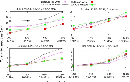
The configuration details of the experiments are summarized in Figure 2.6. Every row represents a subset of experiments where a box size is used to partition four different domains. As the domain size increases, so does the total number of boxes and parallel client/server processes. By default, we use the minimum number of Titan nodes to hold the client and server processes. However, because DART [24], on which DataSpaces is built, utilizes remote-direct-memory-access (RDMA) to transport data, and the memory available for RDMA on each Titan node is about 2GB by default, a large box size or high number of parallel processes means more nodes must be used to host the same number of processes, otherwise DataSpaces crashes. Also note that for AMRZone, Figure 2.6 only shows how many dserver instances are deployed. For all the experiment cases, we consistently use one mserver instance with 15 threads.

(34)

ÿ 12345167891678976

8ÿÿ634ÿ 7345ÿ12634ÿ1678916789862ÿ283457634ÿ76897689768ÿ 1734528634ÿ76897689862ÿ

7297

2972ÿ ÿÿÿÿÿÿÿÿÿ ! !ÿÿÿÿÿÿÿÿÿÿ!ÿÿ ÿÿ!ÿÿÿÿÿÿ !ÿÿ !"ÿÿÿÿÿ !ÿ ÿÿ 17917

972ÿ ÿÿÿÿÿÿÿ ÿÿ !"ÿ!ÿÿÿÿÿÿ !ÿ !ÿÿ "ÿÿÿÿÿÿÿ ÿÿ ""#!ÿÿ!ÿÿ"ÿ !ÿÿÿ 289289

72ÿ "ÿÿÿÿÿ ÿÿ""#!ÿÿ!ÿÿÿÿÿ"ÿ !ÿ"#ÿÿÿÿÿÿ"ÿ ÿ !ÿ"#!ÿÿÿÿ"#!ÿ !ÿ ÿ797ÿ

972ÿ #ÿÿ"ÿÿ"ÿÿ!ÿÿ"#!ÿÿÿÿ"#!ÿ !ÿ$!ÿÿ#ÿ"ÿÿ#ÿ"ÿ! !ÿÿ#ÿ!"ÿ"ÿ

Figure 2.6 Configuration details for the scalability comparison experiments. The row header denotes four domain sizes and the column header gives four partition sizes. The format,$B$C($N) /$S($N), denotes the total number of boxes(B), the total number of parallel client processes(C), the total num-ber of client nodes(N), the total numnum-ber of DataSpaces server or AMRZone dserver processes(S) and the total number of server nodes(N).

(35)

achieves a better result (less increased execution time while more compute resources are devoted to process a larger domain size), compared to DataSpaces. Based on these results, we consider on averageour framework’s performance is comparable with DataSpaces.

2.4.2 Performance over AMR Data

Experiments in this section are aimed at evaluating the write/read performance and workload distribution of AMR boxes at the server space of our framework. First, we use the 2D AMR datasets generated by BISICLES [20], a large-scale Antarctic ice sheet modeling code for climate simulation. Then, to have a baseline for comparison, we also include experiments over 2D double-precision synthetic uniform data with similar configurations. The testing programs know the exact coordinates of boxes. Figure 2.8 gives the detailed information about the experiments over these two datasets.

The BISICLES-generated datasets consist of double-precision values and are 1GB in size. Each dataset has 5 levels, with a total of about 6,700 boxes. To create larger datasets for testing performance, different dataset sizes are created by expanding all boxes of a time-step 8, 16, 32 and 64 times, respectively. So the total number of boxes in a time-step doesn’t change. So an original 1GB dataset is expanded 8, 16, 32 and 64 times, respectively. During this expansion, we ensure that the relative positions of the boxes to their adjacent levels does not change. In each experiment, 512, 1024, 2048 and 4096 parallel processes (based on the client APIs of AMRZone) are used to write/read 10 time-steps of data (recall, each write/read is based on one AMR box). On the server side, we consistently use 1 mserver process with 15 threads and the minimum number of nodes to host those client and dserver processes.

In each of these AMR data related experiments, the workload assignment policy makes each client process have a similar amount of data to write/read. This means that some processes may be assigned a few big boxes, while others may be assigned more boxes of smaller sizes. Although still not completely balanced, compared to assigning each process a similar number of boxes, this approach could achieve a more balanced workload distribution between client processes, thus improving performance.

(36)

01213452ÿ7897ÿÿ7ÿ7ÿ7ÿÿÿÿ87ÿ

ÿÿ ÿ !"ÿ #ÿ

$"%&!"'(ÿ)ÿ$"*&!"'(ÿÿ +"#%& #'(ÿ)ÿ+"#*& #'(ÿ "+#%&"'(ÿ)ÿ"+#*&"'(ÿ#+, %&"$ '(ÿ)ÿ#+, *&"$ '(ÿ - .++ÿ)ÿ-/"0ÿ - .++ÿ)ÿ-"/#0ÿ - .++ÿ)ÿ-#/0ÿ - .++ÿ)ÿ-,/.0ÿ

2172ÿ2345ÿ7ÿ

&!". 6!". (ÿ &!". 6 $$! (ÿ !"& $$! 6 $$! (ÿ #& $$! 6!+."(ÿ $"%&!"'(ÿ)ÿ$"*&!"'(ÿÿ +"#%& #'(ÿ)ÿ+"#*& #'(ÿ "+#%&"'(ÿ)ÿ"+#*&"'(ÿ#+, %&"$ '(ÿ)ÿ#+, *&"$ '(ÿ ,"ÿ)ÿ0&"$ 6$"(ÿ ,"ÿ)ÿ"0&$"6$"(ÿ ,"ÿ)ÿ#0&$"6+"#(ÿ ,"ÿ)ÿ0&+"#6+"#(ÿ

Figure 2.8 Configuration details for two sets of AMRZone experiments, one over expanded BISI-CLES AMR datasets, one over synthetic uniform datasets. Row 2, 6 give the dataset size(GB) for one time-step. For the synthetic datasets, it also gives global dimension size. Row 3, 7 give the to-tal number of client processes(C), the toto-tal number of client nodes(N), the toto-tal number of dserver processes(S) and the total number of server nodes(N) for the corresponding time-step. Row 4, 8 give the total number of boxes(B) and box sizes(MB) in the corresponding time-step. For the synthetic datasets, it also gives the dimension size for a box. In row 2 and 4, the values for BISICLES datasets are average ones.

could cause noticeably more network transmission overhead. Thus, when reviewing the results of the two sets of experiments, it is more appropriate to compare the two sets to each other, rather than comparing all experiments of a single set together.

Figure 2.9 shows the results of the experiments. As expected, the performance over AMR data is worse than the performance over the uniform synthetic data. This could be attributed to the unbalanced workload distribution for client processes when writing/reading AMR datasets. In the worst case (reading an 8GB dataset), AMR data related tasks demand more than 36% additional execution time. In the best case (writing a 64GB dataset), they only need about 2% more additional execution time. There are three cases in which AMR data coupled tasks take more than 10% additional time: writing/reading an 8GB dataset (29%, 36%), and writing a 32GB dataset (11%). A possible explaination for the two 8GB AMR data related cases taking a noticeably higher percentage of additional time is that, the box size of the 8GB synthetic data domain is small, making write/read operations very efficient; therefore, the two perform comparatively worse. In all other cases (5 out of 8), AMR data coupled writes/reads require no more than 10% additional time. Considering the unbalanced AMR boxes distribution on the client processes (the biggest box size is 17 times larger than the smallest one), we believe AMRZone’s performance over real AMR datasets to be comparable with its performance over uniform mesh, thus satisfactory.

(37)

Figure 2.9 Results of boxes write/read performance testing for AMRZone over real AMR datasets, with comparisons on synthetic uniform data, totally 10 time-steps. In the worst case, AMR data related task demands more than 36% additional execution time, in the best case it is 2% more. In 5 cases (out of 8), AMR data coupled write/read needs less than 10% more time. Note these arenot

weak scaling testings.

ÿ

123ÿÿ5678ÿ6923ÿÿ678ÿ 723ÿÿ718ÿ 923ÿÿ98ÿ

ÿ

ÿ ÿ

ÿ

!

ÿÿ

ÿ

"ÿ

ÿ

"ÿ

ÿ

#6ÿ

"ÿ

ÿ

#ÿ

ÿ

$ÿ

ÿ

"ÿ

ÿ

(38)

number of processes. However, the min, avg, median, Q1, and Q3 are quite similar to each other for all types of processes numbers, which indicates a good overall balance. Considering that, for the AMR dataset, the biggest box size is 17 times larger than the smallest one, we believe AMRZone’s workload assignment policy on the server side produces satisfactory results.

2.4.3 Performance of Spatially Constrained Interaction Coupled with AMR Data

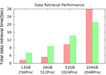
In this section, we evaluate the performance of AMRZone under a more complicated data sharing scenario: retrieving the data (or AMR boxes) of specific spatial regions of interest. The datasets are the same collection of BISICLES’s 1GB time-steps used in the previous subsection (Section 2.4.2). In this dataset, the regions that are covered by boxes at finer levels (for instance, level3 and level4) represent spatial areas of greater interest, for example ice sheet grounding lines, calving fronts, and ice streams [20]. Figure 2.1 shows the visualization of one time-step. At the finest level, there are about 4,100 - 4,300 AMR boxes.

In each of the experiments, we expand all the boxes of a time-step by 0, 2, 4 and 8 times respectively, similar to what is done in Section 2.4.2. Moreover, we first write 10 time-steps of data to the server space, then use 256, 512, 1024 and 2048 parallel processes (based on the client APIs of AMRZone) to perform spatially constrained data retrievals over the staged time-steps one by one. The processes could represent potential data analytics applications. The coordinates of AMR boxes at the finest level are used by the client processes as the spatial query condition to perform the data retrieval. The boxes assignment policy assigns each process a similar number of spatial regions. On the server side, we consistently use 1 mserver process with 15 threads and a minimum number of nodes to host those client and dserver processes. Since in previous experiments AMR data write performance has been evaluated, we only record the execution time of data retrieval in this section.

Before using the coordinates of an AMR box at the finest level for a spatial query, the coordinates need to be properly mapped to the domain of the coarsest level, according to the refinement ratios. Recall that, for AMR data spatial queries, boxes at all levels are retrieved rather than a single level(2.3.3), and more than one box could be refined from a single coarser-level box. So, the total amount of data retrieved may be much larger than the actual size of a time-step. At a single time-step of the 1GB BISICLES datasets, the above designed experiments would retrieve about 26,000 AMR boxes and 13GB data in total. So, for the time-steps that are expanded 2, 4 and 8 times respectively, the final retrieved amount of data is about 26GB, 52GB and 104GB.

(39)

0123425ÿ7893249ÿ232ÿ3425ÿ8ÿ129ÿ00ÿ2323ÿ

ÿ ÿ ÿ ÿ

!"#ÿ$ÿ%!"#ÿÿ !"#ÿ$ÿ%!"#ÿ !"#ÿ$ÿ%!"#ÿ & !&"#ÿ$ÿ&%!&"#ÿ '()*+ÿ$ÿ,-ÿ '()*+ÿ$ÿ-ÿ '()*+ÿ$ÿ-ÿ '()*+ÿ$ÿ-ÿ 8ÿ3425ÿ8ÿ129ÿ00ÿ2323ÿ

ÿ ÿ ÿ ÿ

!"#ÿ$ÿ%!"#ÿÿ !"#ÿ$ÿ%!"#ÿ !"#ÿ$ÿ%!"#ÿ & !&"#ÿ$ÿ&%!&"#ÿ '.()*+ÿ$ÿ-ÿ '.()*+ÿ$ÿ-ÿ '.()*+ÿ$ÿ&-ÿ '.()*+ÿ$ÿ-ÿ

Figure 2.11 Configuration details for two sets of AMRZone experiments over expanded BISICLES datasets, one for spatial constrained data retrieval, one for AMR boxes retrieval. Row 2, 6 give the amount data(GB) retrieved for a time-step. Row 3, 7 give the total number of client processes(C), the total number of client nodes(N), the total number of dserver processes(S) and the total num-ber of server nodes(N) for the corresponding time-step. Row 4, 8 give generally the total numnum-ber of boxes(Boxes) and box sizes(MB) in the retrieved data for a time-step. The values in row 2, 4, 6 and 8 are average ones.

We expand the boxes in the 1GB BISICLES datasets 13, 26, 52, 104 times, write them to the staging space and retrieve the boxes (similar to what is performed in 2.4.2, a read operation is provided the exact coordinates of a box, and the workload assignment policy assigns each process similar amount of data to read). Figure 2.11 gives detailed information about these experiments.

It is important to point out that neither of the two sets of experiments are weak scaling, because the actualworkload for each process doesn’t remain the same while the dataset size and number of processes increase. Thus, when reviewing the results of the two sets of experiments, it is more appropriate to compare the two sets to each other, rather than comparing all experiments of a single set together.

Figure 2.12 shows the results. For the 13GB, 26GB and 52GB cases, the spatially constrained data retrieval use about 69%, 63%, and 32% less execution time compared to reading the AMR boxes. For the 104GB cases, spatially constrained data retrieval takes about 31% more execution time. An important fact which should be considered before explaining the results is that, the spatial access retrieves about 4 times more boxes than the boxes read (as described earlier). However, when the average box size is relatively small, transmitting an individual box is so efficient that even 4 times more transmissions could still be fast. In addition, a relatively smaller number of processes helps to achieve a more balanced workload distribution. Thus, in the first three cases, the spatial queries have a better performance than reading all the AMR boxes.

(40)

(41)

2048 processes case is 143:37. So for the last case, spatial access endures a noticeable performance downgrade. However, considering the above factors, we believe the spatial AMR data retrieval performance of AMRZone is satisfactory overall.

Finally, it takes about 0.8 seconds for the mserver to build the polytree-based spatial index for the 10 time-step data in these experiments. In fact, because expanding the boxes does not impact the box numbers and relative locations at each level of a time-step, whether the boxes are expanded or not does not influence the efficiency of the index construction. Considering the index is built once and read many times, we believe the result is satisfactory.

2.5

Related Works

In-situ and in-transit data analytics are widely used to avoid the high overhead related to file system I/O. In-transit refers to the approach of moving data from the compute nodes on which a simulation is running to a virtual in-memory space that is constructed by another collection of nodes, and performing various analytics tasks over the space. In-situ means the analytics tasks share the same compute resource as the running simulation. The term “analytics” can denote actions like writing data to storage, feature extraction, indexing, compression, transformation, visualization, etc [73]. Towards supporting these complicated tasks, a number of approaches have been proposed.

Work that does not involve file system I/O usually study how to efficiently move data among nodes and provide various functions to facilitate analytics tasks. EVPath [30] enables users to setup dataflows among compute nodes through which fully-typed data can flow with assigned operators, filers, or routing logic. GLEAN [10] makes data movement topologically-aware and provides functionalities like data subfiling and compression. DataSpaces [25] builds a space-filling curve [50] based index over data in the virtual space, and provides efficient access functions to enable live data of any spatial region can be written to or read from the space. These key features of DataSpaces greatly facilitate runtime data sharing across applications, compared to manually implementing these complex communication behaviors by low level programming standards. Those data sharing scenarios typically consist of multiple heterogeneous and coupled simulation processes dynamically exchanging data on-the-fly [25].

(42)

speed up scientific analysis tasks. Based on DataSpaces, ActiveSpaces [27] supports defining and executing data processing routines in the space. SDS [28] provides efficient scientific data management and query as services.

All above works are for uniform mesh data. Moreover, only DataSpaces can build an explicit online data index and provide a public data access API, which are indispensable features for supporting runtime data sharing across applications. To the best of our knowledge, runtime data sharing across AMR capable applications has not been studied before.

2.6