Performance evaluation of Multidimensional Parabolic Type Problems on distributed computing systems Norma Alias1, Rasiya Anwar1 , Che Rahim Che Teh2, Noriza Satam2, Norhafiza Hamzah2,
Zarith Safiza Abd. Ghaffar2, Roziha Darwis2, Md. Rajibul Islam1,
1 Department of Information Technology, College of Computer and Information Sciences, KSU. 2Department of Mathematics, Faculty of Science, University Technology Malaysia, 81310 Skudai, Johor.
E-mail: [email protected], [email protected]
{Norizasatam, norhafizahamzah, zarithsafiza.ag, roziha.darwis, raziafaiz}@gmail.com, [email protected] ` Abstract
Parabolic Partial Differential Equations (PDE) are well suited to multiprocessor implementation. However, the performance of a parallel program can be damaged by the mismatches between the parallelism available in the application and that available in the architecture. Communication cost, memory requirements, execution time, implementation cost, and others from a problem specific function should be considered to estimate a parallel program. In this paper, we present an optimizing technique called granularity analysis to evaluate the parallel algorithms particularly AGE families without degrading the performances. The resultant granularity analysis scheme is appropriate for developing adaptive parallelism of declarative programming languages on multiprocessors. The results recommend that the proposed method can be used for performance estimation of parallel programs. Red Black Gauss Seidel (GSRB) is selected as the benchmark for the differences numerical methods.
Keywords: Parallel programme, performance evaluation, granularity analysis, multiprocessor, multidimensional parabolic equation, AGE.
1.0 Introduction
All the parallel approaches are based on the non-overlapping subdomain [1, 2]. There is no data swap between the neighboring processors at the iteration (q) but there are inter-processor communications between the iteration (q) and the next iteration (q+1). A typical parallel implementation of a parallel AGE assigns several mesh points to each processor p such that each processor only communicates with its two nearest neighbors [3]. The computations of the approximation solutions in subdomain wp are executed independently. The stopping criteria in the processors p are investigated by measuring the size of the inner residuals. Let us define the residual computed in the processors p. This quantity is kept in the processor's memory between successive iterations and it is checked if the residual is reduced by the convergence criterion. The master processor checked the maximum of local convergence criterion and the iteration stopped when the global convergence criterion is met.
In Evans & Sahimi [4, 5] the discretization of parabolic partial deferential equation is derived from Iterative Alternating Decomposition Explicit Method (IADE) [3, 4, 5] and Alternating Group Explicit Method (AGE) [4, 5]. In Norma et al. [3, 8] the six strategies of parallel algorithms in solving parabolic partial differential equations is implemented. These strategies were found to be more effective using a distributed memory machines. In Alias, Sahimi & Abdullah [8], the Conjugate Gradient on AGE method (AGE-CG) was found to be more convergence and accurate compared to AGE. In this paper, the computational analysis of the proposed strategies is presented by using explicit
block
(
2
×
2
)
. These schemes can be effective in reducing data storage accesses in distributed memory and communication time on a distributed computer systems [3]. This research focuses on the cost communication and computational complexity for these iterative methods [6, 9]. All the parallel strategies have been developed to runs on a cluster of workstations based on Parallel Virtual Machine environment [10, 11, 12].As the AGE class is fully explicit its feature can be fully utilized for parallelism [4]. Firstly, Domain is distributed to p subdomain by the master processor. The partitioning is based on data decomposition technique. Secondly, the subdomain p of AGE_BRIAN and AGE_DOUGLAS methods are assigned into processors in block ordering [7, 8].The domain decomposition for AGE_BRIAN and AGE_DOUGLAS methods are implemented in four and five time level, respectively. The communication schemes among the slave processors are needed for the computations in the next iterations [10]. The parallelization of AGE_BRIAN and AGE_DOUGLAS are achieved by assigning the explicit block
(
2
×
2
)
in this way and proved that the computations involved are independent between processors. The parallelism strategy is straightforward and the domain is distributed to non over lapping subdomain[1,9]. Based on the limited parallelism, this scheme can be effective in reducing computational complexity and data storage accesses in distributed parallel computer systems [6,11]. The iterative procedure is continued until convergence is reached.2.0
Fine and Coarse-grain ParallelismComputational grid for high performance computing is the current research focus of computer science [2, 11]. Moreover, the performance analysis and evaluation of parallel programs are crucial in grid computing platform. According to [12-17], granularity analysis of parallel program is one of the key technologies in parallel computing.
As hardware components become more powerful and less expensive, parallel processing has become an indispensable means for achieving higher performance. From the well-known Amdahl’s law [9], software issues are very critical in such parallel systems. Due to the added complexity in multiple system components, the interaction between software and hardware becomes more complicated. For example, it is no longer adequate just to manage register sets, to decrease operation strength, and to pass parameters between procedures effectively. We analysed one of the more complex issues in this study, such as determining the granularity in order to estimate the performances of the parallel algorithms.
without communication with other processes. In parallel computing, granularity is a qualitative measure of the ratio of computation to communication [14, 15]. Computational times are normally separated from communication times by synchronization events. Fine grain and coarse grain algorithms are the two extremes for this [9, 18]. In Fine-grain Parallelism, comparatively small quantities of computational work are done between communication events, low computation to communication ratio, facilitates load balancing, implies high communication overhead and fewer opportunity for performance improvement and if granularity is too fine it is possible that the overhead required for communications and synchronization between tasks takes longer than the computation. On the other hand, in Coarse-grain parallelism, comparatively large amounts of computational work are done between communication/synchronization events, high computation to communication ratio, involves more chances for performance boost and harder to load balance efficiently [9]. The most competent granularity is dependent on the algorithm and the hardware environment in which it runs [12, 14]. In most cases the overhead associated with communications and synchronization are high relative to execution speed so it is beneficial to have coarse granularity. Fine-grain parallelism can help reduce overheads due to load imbalance [18].
In this paper we discuss some of those performances analysis metrics and especially a short explanation about granularity. We concentrate on multidimensional parallel equations especially AGE families only. How granularity helps to evaluate the performances on parallel computing platform are illustrated. Experimental results show the importance of granularity is to obtain the performances of different multidimensional parallel algorithms.
In this research, one, two and three dimensional parabolic problem had been considered for the application of numerical methods [3,4,5].
3.0 Granularity 3.1 Parallel Program Execution Time
According to Foster I. [21], parallel program execution time can be define as the time that elapses from the initial starts by master hosts until the last slaves accomplished the task allocated. In every execution of a parallel program, the timing being measured is the decomposition of computation, communication and idle time [22, 23] .
idle T comm T comp T para
T = + + (1)
para
T is defined as overall time needed for execution of parallel program and can be calculated by adding time for computation,
)
(Tcomp and time for communication, (Tcomm)as well as idle times Tidle.This definition of parallel execution time is useful in measuring communication cost, granularity as well as other parallel performance evaluation, namely speedup, efficiency, effectiveness and temporal performance. The usage of Tpara for the analysis of communication cost is as shown in Table 1, 2 and 3. Additionally, the parallel performance evaluation is shown in Table 7, 8 and 9.
3.2 Computation time and communication time ratio Scientists who work with parallel architectures define the ratio between the computation time and the communication time as the granularity of an application. This comes from the fact that in traditional algorithms (i.e., synchronous algorithms, iterative or not), periods of computation are typically separated from periods of communication by synchronizations. However, dealing with granularity, there are no more synchronizations, thus that traditional definition is not very appropriate. In order to be scalable, an algorithm must be coarse grained [4] 18, i.e., have long computation parts without communications. That is to say, messages must be gathered in order to decrease the number of communications. The granularity of parallel algorithm are investigated using coarse grain of multisplitting method. On the other hand, even though an algorithm has been designed to be coarse-grained, the ratio between the computation time and the communication time may affect its execution times in a given computing context. Hence, in our opinion, this ratio is more important than the notion of the granularity of an application. The main reason lies in the fact that the granularity definition does not involve the speed of the interconnection network which affects the communication time.
4.0 Granularity Analysis
Many metrics are used throughout the performance evaluation of parallel programs [1, 2, 9, 15, 24]. Perhaps the simplest and most intuitive metric of parallel performance are the parallel run time. It is the time from the moment when computation starts to the moment when the last processor finishes its execution. The parallel run time is composed as an average of three different components: computation time, communication time and idle time [14]. (Tcomp) is the time spent on performing computation by all processors, (Tcomm)is the time spent on sending and receiving messages by all processors. Tidle is when processors stay idle. The problem with parallel run time is that it does not account for the resources used to achieve the execution time. Specifically, if one were to indicate that the parallel run time of a program, which took 10s on a serial processor, is 2s, we would have no way of knowing whether the parallel program (and associated algorithm) performs well or not. The second metric is scalability. The property of a program to adapt automatically to a given number of processors is called scalability [1]. Scalability is more sought after than efficiency (ire., gain of computing time by parallelism) on any specific architecture/topology. Another one is speedup. Speedup is the ratio of the running time on a single processor to the parallel running time on p processors [1, 6, 3]. In other word, the ratio of two program execution times, particularly when times are from execution on 1 and p nodes of the same computer. Speedup is usually discussed as a function of the number of processors and the problem size.
only want to measure flops (floating point operations per second), others only want to measure speedup. Actually, only wall clock time counts for a parallel code. The parallel efficiency tells us how close our parallel implementation is to the optimal speedup. The efficiency is a measure of hardware utilization, equal to the ratio of speedup achieved on p processors to p itself.
The numerical efficiency compares the fastest sequential algorithm with the fastest parallel algorithm implemented on one processor via the relationship. Load balance also a metric to evaluate the performance of parallel programs. The equal distribution the computation workload on all processors is called load balance [1]. Statistic and dynamic are the two types of opportunities to achieve a load balance. Effectiveness is used to calculate the speedup and the efficiency [6] . It also can be said that the efficiency of a parallel program divided by the execution time. Temporal performance is a parameter to measure the performance of a parallel algorithm [3, 6]. The cost of solving a problem by the parallel system is another one term, which is regularly used in the performance estimation of parallel programs. The cost is generally defined as a product of the parallel run time and the number of processors.
We need to evaluate the run time of sequential and parallel programs during experimental performance estimation according to the above brief sketch of different performance metrics. Granularity is a qualitative estimation of the ratio of computation to communication in parallel computing [12-17]. In this study parallel performances through granularity are shown on various multidimensional parallel algorithms.
5.0 Parallel Performance Measurement
A study of granularity is important if one is going to choose the most efficient architecture of parallel hardware for the algorithm at hand. In general the granularity of a parallel computer is defined as a ratio of the time required for a basic communication operation to the time required for a basic computation operation [15], and for parallel algorithms as the number of instructions that can be performed concurrently before some form of synchronization needs to take place.
As we can demonstrate that, granularity G of a parallel algorithm can be defined as the ratio of the amount of computation (Tcomp) to the amount of (Tcomm) within a parallel algorithm implementation (G=(Tcomp)/(Tcomm)) [14][15]. This definition of granularity will be applied in this paper.
Therefore to analyse the granularity of a single process the above definition will be utilised executing on the single processor and for the entire program with total communication and computation times of all processors. With having this goal we described the overhead function. The overhead function is a function of problem size and the number of processors and is defined as follows [24]:
W p T p p W o
T ( , )= * − (2)
Where W denotes the problem size, Tp denotes time of parallel program execution and p is the number of processors. The problem size is defined as the number of basic computation operations required to solve the problem using the best serial algorithm. Let us assume that a basic computation operation takes one unit of time. Thus the problem size is equal to the time of
performing the best serial algorithm on a serial computer. Based on the above assumptions after rewriting the equation (2) we obtain the following expression for parallel run time:
p p W o T W p
T = + ( , ) (3)
Then the resulting expression for efficiency takes the form:
W p W o T E
) , ( 1
1
+ =
(4)
Recall that the parallel run time consists of computation time, communication time and idle time. If we assume that the main overhead of parallel program execution is communication time and the idle time can be added to the communication time during run time measurement then equation (4) can be rewritten as follows:
W comm total T E
_ 1
1
+ =
(5)
The total communication time is equal to the sum of the communication time of all performed communication steps. Assuming that the distribution of data among processors is equal then the communication time can be calculated using equation Ttotal_comm= p * (Tcomm). Note that the above is true when the distribution of work between processors and their performance is equal. Similarly, the computation time is the sum of the time spent by all processors performing computation. Then the problem size W is equal to p * (Tcomp). Finally, substituting the problem size and total communication time in equation (5) by using above equations we get:
1 1 1
1
1 1
+ = + = +
=
G G
G comp T
comm T E
(6)
It means that using granularity we can calculate the efficiency and speedup of parallel algorithms. So, it is possible to evaluate a parallel program using such metrics like efficiency and speedup by executing only a parallel version of a program on a parallel computer.
6.0 Numerical Results and Discussion 6.1 Numerical Analysis
Sufficient accuracy is needed as numerical methods continuously being applied in various fields. Thus, any selection of appropriate method for problem solving should consider the errors that definitely will affect the outcomes. By the mean of numerical analysis, the level of accuracy achieved and appropriate number of iterations should be taken into consideration. Numerical analysis is resulting from the sequential execution of GSRB and AGE method is shown in Table 1, 2 and 3.
as problem size increase AGE method shows significance performance improvement and produce better result than classical GSRB iterative method.
6.2 Communication cost
Communication exists in any computation that takes into account the use of more than one processor. Communication session that is established during the process of data exchange among processors affects the overall parallel execution time. Communication cost is total number of communication operation needed during the execution of one parallel algorithm. Therefore, by analyzing the communication cost, the rate of communication activities exist and time allocated for communication in solving multidimensional parabolic problem. The communication cost results for one, two and three- dimension problem are as shown in Table 4, 5 and 6 below,
Table 1-3 depicts the ability of AGE_BRIAN and AGE_DOUGLAS to reduce communication cost compared to GSRB in solving multidimensional problem. Low communication rate for the usage of AGE_BRIAN method continues for two- and three-dimensional problem as it is superior compared to the other two AGE_DOUGLAS and GSRB.
6.3 Computational complexity
Computational complexity depends on total number of arithmetic operations exist in the problem being modeled. Instead of arithmetic operations, the use of trigonometry functions such as sinus, cosines and tangent as well as square root function will also affecting the computational complexity. Different method results in different complexity as they have different rate of ability to iterate until meet the convergence criterion. In this research, the analysis of computational complexity for multidimensional problem under consideration is as shown in table 7, 8 and 9. Analysis of computational complexity shows the bright potential of AGE family method (DOUGLAS and BRIAN) same as in communication cost evaluations. In terms of rank, AGE_BRIAN will be the best method to choose for problem solution and this followed by AGE_BRIAN method. GSRB classical iterative method will serve as benchmark to ease the comparison among methods used.
6.4 Evaluation of Granularity
The performance evaluation of parallel computing has obtained based on the numerical results, in respect of communication and computational ratio [25]. For this experiment we have used Pentium PC with Core2Duo processor each and PVM were used as the software environment [10, 11, 25].
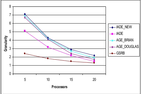
According to [15], The experiment results of AGE_BRIAN, AGE_DOUGLAS and GSRB are summarised in Tables 1-3. Here among all these methods, its noticeable that granularity is decreasing for all in terms of increasing number of processors (see Fig. 1). Because of granularity depends of computational time, communication time and idle time. Hence in Fig. 1 and Table 4 show that granularity decreasing while communication time decreasing as well. Therefore, from the comparative performance evaluation through granularity, it’s shown that AGE_BRIAN producing more granularities with lower computational time than
AGE_DOUGLAS method. Furthermore, AGE_BRAIN producing higher granularity in respect of increasing processing units among all the other methods shown in table 7-9.
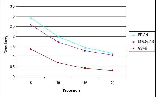
Fig. 2 and Fig. 3 show the granularity distribution of (600×600) matrix and (1000×1000) matrix multiply program executed on 20 parallel processing nodes. Granularity analysis of two-dimensional AGE_BRIAN, AGE_DOUGLAS and GSRB in respect of the number of processors using (600×600) and (1000×1000) sizes of matrices respectively. Here granularity decreases while number of processors increases. Again granularity increases while the size of matrices increases. According to the granularity distribution, we may exploit the critical point between sequence execution and parallel execution, and design optimized parallel task scheduling strategy.
Fig. 4 and Fig. 5 show the granularity analysis of three-dimensional AGE_BRIAN , AGE_DOUGLAS, GSRB with having (100×100×100) and (140×140×140) matrix. Here also the same results have come out as same as Table 6, except BRIAN and DOUGLAS with having (100×100×100) matrix size. In Fig. 4 – Fig. 5 shown that granularity were decreasing for AGE_BRIAN, AGE_DOUGLAS and GSRB while the number of processing unit increasing. Therefore, normally from all the tables it’s shown that granularity decreasing in respect of increasing processing units.
0 1 2 3 4 5 6 7 8
5 10 15 20
Processors
G
ra
nu
la
rit
y
IADE_NEW IADE AGE_BRIAN AGE_DOUGLAS GSRB
Fig. 1: Granularity analysis of one-dimensional AGE_BRIAN, AGE_DOUGLAS, GSRB versus number of processors
0 0.5 1 1.5 2 2.5 3
5 10 15 20
Processors
G
ra
n
u
la
ri
ty BRIAN
DOUGLAS GSRB
0 1 2 3 4 5 6 7
5 10 15 20
Processors
G
ra
n
u
la
ri
ty BRIAN
DOUGLAS GSRB
Fig. 3: Granularity analysis of two-dimensional AGE_BRIAN, AGE_DOUGLAS and GSRB versus number of processors using (1000 × 1000) sizes of matrices.
0 0.2 0.4 0.6 0.8 1 1.2 1.4 1.6 1.8 2
5 10 15 20
Processors
G
ra
nu
la
ri
ty BRIAN
DOUGLAS GSRB
Fig. 4: Granularity analysis of three-dimensional AGE_BRIAN , AGE_DOUGLAS and GSRB versus number of processors using (100 × 100 × 100) sizes of matrices.
0 0.5 1 1.5 2 2.5 3 3.5
5 10 15 20
Processors
G
ra
nu
la
rit
y BRIAN
DOUGLAS GSRB
Fig. 5: Granularity analysis of three-dimensional AGE_BRIAN, AGE_DOUGLAS and GSRB versus number of processors using (140×140×140) sizes of matrices.
From these results, it is quite clear that granularity can be applied as one of the performance metrics of parallel algorithms. In the experiments it’s shown that multidimensional of AGE methods perform well in parallel environments. The granularity changes in respect of number of processing units, computational time,
communication time, idle time and even matrix size and dimensionality of the parallel methods. Thus, from this study it’s come out that granularity can be used significantly for the performance evaluation of the parallel strategies and performs to obtain the results that AGE_BRIAN method performs better performance among other multidimensional parallel methods. The results have proved that granularity can play a vital role to estimate the parallel performances of multidimensional parallel methods. PVM is used in the experiments of this study as a time-saving software tools in terms of message latency and communication time [10, 11, 25].
7.0 Conclusion
The paper presents an analytical study to evaluate the numerical and parallel performances of different parallelization methods. The AGE_BRAIN is the alternative and most suitable method for the solution of multidimensional parabolic problem among AGE families. This is based on results depicted in Table 1-10 which shows the comparison among AGE families. This clearly shows AGE_BRIAN is the best method among AGE families. For one, two and three dimensional problem, experimental test had been done among the standard multidimensional GSRB methods. AGE BRAIN shows significant performance achievement as shown in Table 7-9 compared to two other methods being tested. Thus, for the solution of multidimensional problem, AGE type of BRAIN is the most suitable iterative method as it converged faster than AGE_DOUGLAS and GSRB Since performance analysis is the most important branch of high performance computing research, the measurement is important aspect to be concern. Therefore, this study deals with ry the use of an idea as granularity in the estimation of parallel programs. The results acquired from the analysis, recommend that the presented method can be used for performance assessment of parallel programs. Experimental results confirm that granularity measurement can be use for all investigated algorithms. However, it cannot be used for algorithms with speedup inconsistency. The algorithms which do not require frequent communication provides better results.
This research can be extended in future through improving the prediction accuracy and solving undetermined operations in programs. By the experimental outcomes it is confirmed that the offered method can be used for all studied algorithms [14, 15, 16, 17].
Acknowledgment
Appreciated to the King Saud University, Riyadh, Saudi Arabia for the research collaboration and financial support of the publication.
Reference
[2]
Jacques Mohcine Bahi, Sylvain Contassot-Vivier, Raphaël Couturier, Parallel Iterative Algorithms From Sequential to Grid Computing, Chapman & Hall/CRC, Taylor & Francis Group, Boca Raton, FL,2008, p.75.[3]
Norma Alias, Sahimi, M.S., and Abdullah, A.R., The AGEB Algorithm for Solving the Heat Equation in Two Space Dimensions and Its Parallelization on a Distributed Memory Machine. Proceedings of the 10th European PVM/MPI User's Group Meeting: Recent Advances In Parallel Virtual Machine and Message Passing Interface. Venice: Italy, pp. 214-221, 2003.[4]
Evans, D.J., Sahimi, M.S. The Alternating Group Explicit (AGE) Iterative method for Solving Parabolic Equations II: 3 Space Dimensional Problems. International Journal Computer Mathematic.26:117-142 (1989).[5] Evans, D.J., Sahimi, M.S.,The Alternating Group Explicit Iterative Method (AGE) to Solve Parabolic and Hyperbolic Partial Differential Equations. In Annual Review of Numerical Fluid Mechanics and Heat Transfer, Vol. 2. Hemisphere Publication Corporation, New York Washington Philadelphia London .1989.
[6]
Norma Alias, Roziha Darwis, Noriza Satam, Zarith SafizaAbd. Gaffar, Norhafiza Hamzah, Md. Rajibul Islam and Tan Yin San, “Parallel Iterative Block and Direct Block Methods for 2-Space Dimension Problems on Distributed Memory Architecture”, in Proc. of 6th International Conference of Information Technology in Asia 2009 (CITA’09), Sarawak, Malaysia, July 6-9, 2009, pp. 170-174.
[7]
Louis A. Hageman, David M. Young, Applied Iterative Methods, Academic, New York, 1981.[8]
Norma Alias, Sahimi, M.S., and Abdullah, A.R., Parallel Strategies For The Iterative Alternating Decomposition Explicit Interpolation-Conjugate Gradient Method In solving Heat Conductor Equation On A Distributed Parallel Computer Systems. Proceedings of The 3rd International Conference On Numerical Analysis in Engineering. 3: 31—38. 2003.[9]
Cosnard M. and Trystan D., Parallel Algorithms and Architectures, International Thomson Publishing Company, London, 1995.[10]
Blaise Barney, Lawrence Livermore National Laboratory, Introduction to Parallel Computing [Available Online]: https://computing.llnl.gov/tutorials/parallel_comp/[11]
Norma Alias, Noriza Satam, Roziha Darwis, NorhafizaHamzah, Zarith Safiza Abd. Ghaffar, Md. Rajibul Islam, “Mathematical simulation for 3-Dimensional Temperature Visualization on Open Source-based Grid Computing Platform”, in Proc. of International Conference on Computer Research and Development (ICCRD 2009) Perth, Australia, July-10-12, pp. 553-559, 2009.
[12]
Wei-guang Qiao and Guosun Zeng, The Granularity Analysis of MPI Parallel Programs’, Lecture Notes in Computer Science (LNCS) 3032, Springer-Verlag Berlin Heidelberg pp. 192–195, 2004.[13]
Ding-Kai Chen, Hong-Men Su and Pen-Chung Yew, The impact of synchronization and granularity on parallel systems, Proceedings of the 17th annual international symposium on Computer Architecture,Pages: 239 – 248, vol-18 (3a), 1990.[14]
Jan Kwiatkowski, Evaluation of parallel programs by measurement of its granularity, R. Wyrzykowski et al. (Eds.): PPAM 2001, LNCS 2328, pp. 145–153, 2002.[15]
Kwiatkowski J., Performance Evaluation if ParallelPrograms, in Proc. of the International Conference Parallel Processing and Applied Mathematics PPAM’99, Kazimierz Dolny, Poland 1999, pp. 75-85
[16]
Tian Xinmin, Wang Dingxing, Shen Meiming, ZhengWeimin and Wen Dongchan, Granularity Analysis for Exploiting Adaptive Parallelism of Declarative Programs on Multiprocessors, Journal of Computer Science & Technology, 9(2): 144-152 (1994).
[17]
W. Hui, Visualizing Object/Method Granularity for Program Parallelization, M.Sc. Thesis, Department of Computing Science, University of Alberta, 1998.[18]
D. Rabideau, A. Steinhardt, Fast subspace tracking usingcoarse grain and fine grain parallelism, in Proc. of the International Conference on Acoustics, Speech, and Signal Processing (ICASSP - 95), vol. 5, pp. 3211-3214, 1995.
[19]
Evans, D.J., Sahimi, M.S., The Alternating Group Explicit (AGE) Iterative Method for Solving Parabolic Equations I: 2-Dimensional Problems. Intern. J. Computer Math. 24:311-341 (1988).[20]
Sahimi, M. S. and Muda Z., An iterative explicit method for parabolic problems with cylindrical symmetry-increased accuracy on Non-Uniform Grid. Pertanika J., 12: 413-419 (1989).[21]
S. D. Conte, Elementary Numerical Analysis. McGraw-Hill, 1965.[22]
Foster I., Designing and Building Parallel Programs. Addison-Wesley Longman Publishing Co., Inc. 1995.[23]
Jeffrey S. Vetter and Michael O. McCracken, StatisticalScalability Analysis of Communication Operations in Distributed Applications, Proceedings of the eighth ACM SIGPLAN symposium on Principles and practices of parallel programming pp. 123 – 132, 2001.
[24]
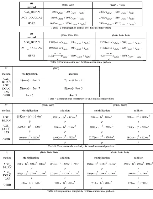
Grama A.Y., Gupta A., Kumar V., Isoefficiency, Measuring the Scalability of Parallel Algorithms and Architectures, IEEE Parallel & Distributed Technology, August 1993, pp. 12-21.Table 1: Sequential Analysis of GSRB and AGE method for the solution of 1-dimensional parabolic heat conduction problem (MSE=mean square error, RMSE = root mean square error, r=acceleration parameter and ∆x= grid meshes at x-axis)
m (600× 600) (1000×1000)
method GSRB AGE_DOUGLAS AGE_BRIAN GSRB AGE_DOUGLAS AGE_BRIAN
Execution time
(second) 40.1592 35.6894 33.8854 157.6732 143.2267 138.9811
Iteration 300 150 130 622 230 200
MSE 3.07461E-12 3.07398E-12 3.07166E-12 2.4482E-12 2.4416E-12 2.4396E-12
RMSE 1.0151E-11 1.0116E-11 1.0120E-11 2.4482E-12 8.0597E-12 8.0722E-12
r - 0.95 0.99 - 1.6 1.6
x
∆ 1.67E-3 1.67E-3 1.67E-3 1.00E-3 1.00E-3 1.00E-3
y
∆ 1.67E-3 1.67E-3 1.67E-3 1.00E-3 1.00E-3 1.00E-3
Table 2: Sequential Analysis of numerical methods for the solution of 2-dimensional parabolic heat conduction problem. ( ∆y= grid meshes at y-axis)
Table 3: Sequential Analysis of GSRB and AGE method for the solution of 3-dimensional parabolic heat conduction problem ( ∆z= grid meshes at z-axis)
method Communication cost
AGE_BRIAN 3000tdata +1500(tstart+ tidle)
AGE_DOUGLAS 3000tdata +1500(tstart+ tidle)
GSRB 7200tdata+ 3600(tstart + tidle)
method GSRB AGE_BRIAN AGE_DOUGLAS
Execution time
(second) 154.4432 48.743 50.0625
Iteration 600 250 250
MSE 1.5921E-9 1.5921E-9 1.5921E-9
RMSE 1.9846E-7 1.9846E-7 1.9845E-7
r - 0.8 0.6
x
∆ 1.3889E-6 1.3889E-6 1.3889E-6
m (100×100×100) (140×140×140)
method GSRB AGE_DOUGLAS AGE_BRIAN GSRB AGE_DOUGLAS AGE_BRIAN
Execution time (second)
282.95 221.06 216.34 558.93 710.42 650.8
Iteration 760 125 115 650 120 110
MSE 4.117E-5 6.5350E-13 6.5119E-12 1.2012E-14 1.2009E-14 1.2012E-14
RMSE 1.0151E-11 1.0116E-11 1.0120E-11 2.4482E-12 8.0597E-12 8.0722E-12
r - 1 0.8 - 1.1 1.2
x
∆ =∆y 1.0E-2 1.0E-2 1.0E-2 7.143E-3 7.14E-3 7.143E-3
z
Table 4: Communication cost for one-dimensional problem
m
method (600×600) (1000×1000)
AGE_BRIAN 1560mtdata+ 780(tstart+ tidle) 2400mtdata+1200(tstart + tidle) AGE_DOUGLAS 1800mtdata + 900(tstart + tidle) 2760mtdata+1380(tstart + tidle)
GSRB 6000mtdata+ 3000(tstart+ tidle) 7464mtdata + 3732(tstart + tidle)
Table 5: Communication cost for two-dimensional problem
m
method (100×100×100) (140×140×140)
AGE_BRIAN 1380(m× m)tdata+ 690(tstart+ tidle) 1320(m× m)tdata+ 660(tstart+ tidle) AGE_DOUGLAS 1500(m× m)tdata+ 750(tstart+ tidle) 1440(m× m)tdata+ 720(tstart+ tidle)
GSRB ) 4560( )
2 (
9120 m× m tdata + tstart+ tidle ) 3900( )
2 (
7800 m× m tdata + tstart +tidle
Table 6: Communication cost for three-dimensional problem
m
(100)method multiplication addition
AGE_
BRIAN 18(cons)+10m+5 7(cons)+8m+5 AGE_
DOUG LAS
7 12 ) (
21cons + m+ 11(cons)+ 8m+5
GSRB 6m+ 5 4m+3
Table 7: Computational complexity for one-dimensional problem
m
(600×600) (1000×1000)method Multiplication addition multiplication addition
AGE_
BRIAN p
m
m 1)2 1040 2
(
1832 − +
p m
m 1)2 1690 2
( 3380 − +
p m m 1)2 1600 2 (
2800 − +
p m m 1)2 2600 2 (
5200 − +
AGE_ DOUG
LAS p
m m 1)2 1500 2
(
3000 − +
p m
m 1)2 1950 2
(
3900 − +
p m
m 1)2 2300 2
( 4600 − +
p m m 1)2 2990 2 (
5980 − +
GSRB
p m m 1)2 7000 2 (
5000 − +
p m m 1)2 7500 2 (
5500 − +
p m
m 1)2 8708 2
( 6220 − +
p m m 1)2 9330 2 (
6842 − +
Table 8: Computational complexity for two-dimensional problem
m
(100×100×100) (140×140×140)method Multiplication addition multiplication addition
AGE_
BRIAN p
m m m 1)3 3450 3 1610 2 (
1380 − + +
p
m m m 1)3 2875 3 1725 2 (
2875 − + +
p
m m m 1)3 3300 3 1540 2 (
1320 − + +
p
m m m 1)3 2750 3 1650 2 (
2750 − + +
AGE_ DOUG
LAS p
m m m 1)3 3750 3 2250 2 (
2376 − + +
p
m m m 1)3 3125 3 1875 2 (
3125 − + +
p
m m m 1)3 3600 3 2160 2 (
2280 − + +
p m m 1)3 1800 3 (
3000 − +
GSRB
p m m 1)3 10640 3 (
11400 − +
p m m 1)3 9120 3 (
9880 − +
p m m 1)3 9100 3 (
9750 − +
p m m 1)3 7800 3 (
8450 − +