Aerodynamic Validation using MER and Phoenix Entry Flight Data.

(1)

Abstract

THOMAS, CASEY. Aerodynamic Validation using MER and Phoenix Entry Flight Data. (Under the supervision of Dr. Robert Tolson.)

Every NASA Mars landing mission has used a 70-degree half-cone forebody,

however with different aft shapes for each mission. To keep with future NASA goals, it is

important to evaluate the aerodynamic database for this forebody design. The purpose of

this thesis is to first assemble the heritage aerodynamic data for this forebody, and then

compare this ground based data with flight data taken from three most reason Mars

entries (MER A, MER B, and Phoenix). The current Mars entry vehicle aerodynamic

database (MEVAD) was updated from the initial Viking wind tunnel data with results

from computational fluid dynamics (CFD) codes. The traditional MEVAD aerodynamic

coefficients of CN, CY, Cm and Cn were used in comparison with the flight derived

coefficients. The metrics for validation were based upon the coefficient differences and

the uncertainty associated with MEVAD. The validation of MEVAD indicated that

coefficients from MEVAD produced slightly higher force coefficients than the

flight-derived coefficients during the second hypersonic instability, which resulted in less than

1 degrees difference in α and β. The difference from the coefficients comparison was

equal to or less than the uncertainty from MEVAD and in the case of the force

coefficients was half the uncertainty from MEVAD. An inconsistency in MEVAD was

suggested by a difference of 2.5 degrees in the resulting α and β determined from the

comparison of the interpolation of the flight derived moment and force coefficients into

MEVAD from 20 second from parachute deployment to parachute deployment for all

(2)

and in the case of Phoenix the Cl corresponded to the change of the total angle of attack

(3)

Aerodynamic Validation using ME R and Phoenix Entry Flight

Data

by Casey Thomas

A thesis submitted to the Graduate Faculty of North Carolina State University

in partial fulfillment of the requirements for the Degree of

Master of Science

Aerospace Engineering

Raleigh, North Carolina

2011

APPROVED BY:

__________________________ _______________________

Dr. Fred Dejarnette Dr. Larry Silverberg

_________________________________________

(4)

Biography

Casey Thomas was born in Northern Hospital of Surry County on August 22,

1983, to Mr. Donald and Gaynell Thomas. He is the older brother of Donna Thomas. He

attended White Plains Elementary School, Gentry Middle School, and North Surry High

School. In high school, he worked at his father’s automobile repair center. It is here

where he became interested in modifying mechanical components for better performance.

After high school, he attended Surry Community College and where he developed an

interest in engineering. He graduated with an Associates in Science from Surry

Community College in 2004. He transferred to the University of North Carolina at

Charlotte where he graduated with a Bachelors of Science Degree in Mechanical

Engineering in 2007. He is currently working at the National Institute of Aerospace and

at NASA Langley Research Center under the supervision of Dr. Robert Tolson. While at

the National Institute of Aerospace he has been attending North Carolina State

University. He plans on graduating with his Masters of Science in Aerospace Engineering

(5)

Acknowledgements

I would like to thank everyone that made this report possible. A special thanks to

Dr. Tolson who guided and inspired me. A special thanks to Professor Blanchard who

pushed me further than I thought was possible. To my family and friends thank you for

(6)

List of Figures

Figure 3.1: Body-axis (XB, YB, ZB) and cruise-axis (XC, YC, ZC) coordinate systems...7

Figure 3.2: Accelerations along the body x-axis for MER A, MER B, and Phoenix....10

Figure 3.3: MER A angular rates in body coordinate system ... 14

Figure 3.4: MER B angular rates in body coordinate system. ... 15

Figure 3.5: Phoenix angular rate components in cruise coordinate system. ... 16

Figure 3.6: MER A angular accelerations in body coordinate system. ... 18

Figure 3.7: MER B angular accelerations in body coordinate system. ... 19

Figure 3.8: Phoenix angular accelerations in body coordinate system...20

Figure 3.9: MER A accelerations in body coordinate system. ... 25

Figure 3.10: MER B accelerations in body coordinate system. ... 26

Figure 3.11: Phoenix acceleration components in cruise coordinate system. ... 27

Figure 3.12: Areodetic altitude and atmospheric relative velocity of the MER A, MER B, and Phoenix entry vehicles...30

Figure 3.13: Total angle of attack from all entry vehicles. ...31

Figure 4.1: MER A Mach and Knudsen numbers for flight exacted and preflight atmospheres...36

Figure 4.2: MER B Mach and Knudsen numbers for flight extracted and preflight atmospheres...37

Figure 4.3: Phoenix Mach and Knudsen numbers for flight exacted and preflight atmospheres...39

Figure 5.1: MER A database force coefficient differences using two atmospheric models...40

Figure 5.2: MER A database moment coefficient differences using two atmospheric models...41

Figure 5.3: MER B database force coefficient differences using two atmospheric models...42

Figure 5.4: MER B database moment coefficient differences using two atmospheric models... 43

Figure 5.5: Phoenix force database force coefficient differences using two atmospheric models... 44

Figure 5.6: Phoenix database moment coefficient differences using two atmospheric models...45

Figure 6.1: MER A atmospheric comparison for CN. ...48

Figure 6.2: MER B atmospheric comparison for Cm. ...49

Figure 6.3: Phoenix atmospheric comparison for Cn. ...50

Figure 7.1: Combination coefficient determination procedure. ...52

Figure 7.2: MER A CN comparison with three methods for determining coefficients. .55 Figure 7.3: MER B CY with three methods for determining coefficients. ...57

Figure 7.4: Phoenix CN with three methods for determining coefficients. ...59

Figure 7.5: MER A Cm with three methods for determining coefficients. ...61

Figure 7.6: MER B Cn with three methods for determining coefficients. ...63

(9)

Figure 7.8: MER A, MER B, and Phoenix rolling moment aerodynamic coefficient, Cl.

...68

Figure 8.1: MER A angle of attack and sideslip angle differences from the combined coefficient method...70

Figure 8.2: MER B angle of attack and sideslip angle differences from the combined coefficient method...71

Figure 8.3: Phoenix angle of attack and sideslip angle differences from the combined coefficient method... 72

Figure 18.1: MER A Earth J2000 to body frame quaternion. ...148

Figure 18.2: MER B Earth J2000 to body frame quaternion. ...149

Figure 18.3: Phoenix PICS to cruise frame quaternion. ...149

Figure 18.4: Aerodynamic coefficient definitions. ...150

Figure 18.5: MER A CY comparison with three methods for determining coefficients. ...151

Figure 18.6: MER A Cn comparison with three methods for determining coefficients. ...152

Figure 18.7: MER B CN comparison with three methods for determining coefficients. ...153

Figure 18.8: MER B Cm comparison with three methods for determining coefficients. .... ...154

Figure 18.9: Phoenix CY comparison with three methods for determining coefficients. ...155

Figure 18.10: Phoenix Cm comparison with three methods for determining coefficients. ...156

Figure 18.11: MER A angle of attack comparison with three methods for determining the angle...157

Figure 18.12: MER A sideslip angle comparison with three methods for determining the angle...158

Figure 18.13: MER B angle of attack comparison with three methods for determining the angle...159

Figure 18.14: MER B sideslip angle comparison with three methods for determining the angle...160

Figure 18.15: Phoenix angle of attack comparison with three methods for determining the angle...161

(10)

List of Tables

Table 3.1 Body coordinate system to IMU frame quaternion. ... 8

Table 3.2 MER A PICS to Earth J2000 DCM ... 21

Table 3.3 MER B PICS to Earth J2000 DCM ... 21

Table 3.4 Distance Components from the IMU to COM in the Body-Axis Frame. .... 23

Table 3.5 Biases by mission... 23

Table 3.6 Misalignments in the rover IMU accelerations. ... 24

Table 3.7 Initial conditions for Mars entry missions in PICS. ... 28

Table 6.1 Moments of inertia and mass. ... 47

Table 7.1 MER A Force coefficient average differences. ... 56

Table 7.2 MER B Force coefficient average differences. ... 57

Table 7.3 Phoenix Force coefficient average differences. ... 60

Table 7.4 MER A moment coefficient average difference. ... 62

Table 7.5 MER B moment coefficient average difference. ... 63

Table 7.6 Phoenix moment coefficient average difference. ... 66

Table 11.1 Force and moment coefficient accuracy for Viking wind tunnel supersonic data...82

Table 11.2 Force and moment coefficient accuracy for Viking wind tunnel transonic data. ... 82

Table 11.3 MER aerodynamic database program uncertainties. ... 88

(11)

Table 11.5 Uncertainties in the static coefficients for transitional and free molecular

flow for MER and Phoenix. ... 92

Table 12.1 Viking wind tunnel data. ... 93

Table 12.2 Viking ballistic range data from PBR at Mach 2 in air. ... 102

Table 12.3 Viking ballistic range data from HFFAF at Mach 2 in air. ... 103

Table 12.4 Viking ballistic range data from HFFAF at Mach 11 in CO2. ... 103

Table 12.5 Viking ballistic range data from HFFAF in air with Reynolds number held constant. ... 104

Table 12.6 Viking ballistic range data from HFFAF in CO2 with Reynolds number held constant. ... 104

Table 12.7 Viking ballistic range data from HFFAF with total angle of attack held constant. ... 105

Table 12.8 Viking flight data from Viking 1. ... 105

Table 13.1 Pathfinder perfect gas aerodynamic coefficients determined from Halis CFD. ... 117

Table 13.2 Pathfinder real gas aerodynamic coefficients determined from LAURA CFD code. ... 119

Table 13.3 Pathfinder aerodynamic database aerodynamic coefficients. ... 120

Table 14.1 MER ballistic range testing... 121

Table 14.2 MER aerodynamic database program aerodynamic coefficients. ... 127

Table 15.1 Phoenix aerodynamic database program aerodynamic coefficients ... 130

(12)

Table 17.1 Pathfinder DAC aerodynamic coefficients. ... 139

Table 17.2 Pathfinder DACFree aerodynamic coefficients. ... 141

Table 17.3 Pathfinder aerodynamic database program aerodynamic coefficients. ... 142

Table 17.4 Pathfinder aerodynamic database program aerodynamic coefficients. ... 143

Table 17.5 MER aerodynamic database program DAC aerodynamic coefficients. ... 144

(13)

Nomenclature

Acom acceleration at the center of mass

Aimu acceleration at the IMU location

A reference area

CA axial force coefficient

Cl rolling moment coefficient

Cm pitching moment coefficient

CN normal force coefficient

Cn yawing moment coefficient

CY side force coefficients

D spacecraft diameter

dbar CO2 hard sphere gas diameter, 4.64e-10 m

g local gravity

gx, gy, gz gravitation components in PICS

h geodetic altitude

J2 second zonal harmonic

Kn Knudsen number

M Mach number

n number density

Na Avogadro's Number, 6.023e26 1/mole

q quaternion

(14)

q2 Y sin(θ/2)

q3 Z sin(θ/2)

q4 cos(θ/2)

time rate of change of the quaternion

P pressure

specific gas constant for CO2, 188.9223

Rarm distance from nose to moment reference location

Rcti position vector from center of mass to the IMU

RMars Mars equatorial radius, 3396200 m

Rpostion position of the spacecraft in PICS

Re Reynolds number

V atmosphere relative velocity

Vint velocity in PICS

Vs speed of sound

Acronyms

AHFFAF Ames Hypervelocity Free-Flight Aerodynamic Facility

APBR Ames Pressurized Ballistic Range

CFHT Continuous Flow Hypersonic Tunnel

CFD Computational Fluid Dynamics

DCM Directional Cosine Matrix

(15)

IMU Inertial Measurement Unit

LAURA Langley Aerothermodynamic Upwind Relaxation Algorithm

LEFTP Langley Eight Foot Transonic Pressure Tunnel

MER Mars Exploration Rover

MEVAD Mars entry vehicle aerodynamic Database

PICS Planet Inertial Coordinated System

MRP Moment Reference Point

MSL Mars Science Laboratory

MST Mach Six Tunnel

UPWT Unitary Plan Wind Tunnel

Greek

α angle of attack

αT total angle of attack

β sideslip angle

λd mean free path of a gas molecule

γ ratio of specific heats, 1.3

ρ density

µ gravitation parameter

ω angular rotation rate of the spacecraft

ωMars rotation rate of Mars

(16)

1. Introduction.

Planetary exploration has been one of humanity's goals since the time of Galileo.

In keeping with this tradition, NASA developed a planetary exploration program. The

NASA planetary exploration program has sent satellites to all planets in our solar system

and has deployed entry vehicles to some. Entry vehicle designs are significantly more

challenging from an engineering point of view because not only do they travel through

space and enter orbit like the satellites, but also they must traverse the atmosphere of the

host planet. The aerodynamics of the entry vehicle becomes critical to mission success in

several ways. For example, by altering the landing location and by dissipating kinetic

energy from planet approach velocity such that parachute deployment is possible.

NASA has landed six entry vehicles on Mars to date. The entry vehicles sent to

Mars have used a 70-degree half-cone angle forebody shape. This forebody shape is to be

used for the entry phase on the upcoming Mars Science Laboratory landing mission.

NASA selected this forebody shape due to its high drag characteristics at hypersonic

velocities. High drag vehicles, such as those with the 70-degree half-cone angle forebody,

facilitate the transfer of planet approach kinetic energy into the atmosphere of the planet,

thus reducing vehicle velocity without additional propulsive maneuvers. Also, the last

two Mars missions landed down track of the predicted landing site, which raised concerns

about the current aerodynamic database1,2. Because of these two reasons and NASA’s

future interest in Mars exploration, it is important to verify the current Mars entry vehicle

(17)

The goal of this thesis is to validate the existing MEVAD using flight data. The

validation is based upon the comparison of flight data from the last few Mars missions,

i.e. MER A, MER B, and Phoenix, and their respective aerodynamic databases. The two

respective aerodynamic databases were used because the bounded static hypersonic

instabilities are functions of velocity and altitude, which are mission dependent3. The

validation was based upon the difference in traditional aerodynamic coefficients, i.e., CN,

CY, Cm, Cn, and Cl. CA is not in the list because it was used for calculating the density and

as a result was not used in the comparison. The metrics of the validation were the

nominal difference in the coefficients as well as the uncertainties associated with the

coefficients from the corresponding aerodynamic database from each mission.

The flight derived aerodynamic coefficients determinations from each mission

require four data quantities, namely, atmospheric relative velocity, accelerations, angular

rates, and density. The atmospheric relative velocity was determined from a trajectory

reconstruction. All three entry vehicles had onboard accelerometers and gyros, which

produced acceleration and angular rate data throughout entry. The atmospheric density

was not measured directly on any of the examined missions. To circumvent the lack of

density measurements, two methods for determining atmospheric properties were

utilized. The first method for determining density utilized a preflight model that was used

for mission planning and the second method derived density from flight data using the

database axial coefficient, CA along with axial acceleration.

The MEVAD contains all of the force and moment coefficients for each Mars

(18)

number (or Knudsen number in the rarefied flow regime). Angle of attack, sideslip angle,

and atmospheric relative velocity are determined from a trajectory reconstruction process.

The Mach number and Knudsen number require a density. As mentioned, two different

methods for determining density are used in this analysis. These methods for determining

density will be discussed later in the report. Section 2 provides a brief summary of the

MEVAD and Appendixes A-G provides a full report on the MEVAD along with tables

for the aerodynamic coefficients.

2. Mars Entry Vehicle Aerodynamic Database.

The MEVAD was created for Viking and was modified for every subsequent

NASA Mars entry mission. The Viking aerodynamic database consisted of ballistic range

and wind tunnel data4,5. Since the Viking era, MEVAD has been updated with

computational fluid dynamics (CFD). In its current state, the MEVAD is a combination

of Viking wind tunnel data for subsonic through supersonic regimes and CFD results

were used for the hypersonic through rarefied flow regimes3. Each mission built around

the core of MEVAD and developed a unique aerodynamic database for mission planning.

Since the Viking era, subsequent additions to the coefficient database included

regions where the entry vehicle is unstable. There are three vehicles instabilities; two

bounded static hypersonic instabilities and one dynamic instability that all Mars entry

vehicles have the possibility of going through during entry. The first in-flight or high

speed bounded static hypersonic instability occurs as a result of the sonic line moving

from the shoulder on the leeside (opposite the windward side) of the vehicle to the nose

(19)

nonequilibrium to equilibrium. This change typically occurs during the transition from

rarefied flow to continuum flow6. The second in-flight or low speed bounded static

hypersonic instability only occurs at low total angles of attack (approximately less than 4

degrees) and results from the sonic line moving back from the nose region to shoulder on

the leeside. The sonic line moves due to the flow enthalpy decreasing in a near

equilibrium gas chemistry regime6. Viking flew at a high total angle of attack

(approximately 11 degrees) so it never experienced the second instability. Each mission

developed its respective mission aerodynamic database because the bounded static

hypersonic instabilities are functions of flow energy and gas chemistry, which are

mission dependent6. The aerodynamic coefficients outside the bounded static hypersonic

instabilities regions are not significantly different between the different aerodynamic

databases and form the core of MEVAD.

The third instability, the dynamic instability, occurs at low Mach numbers (less

than Mach 3.5) and was observed in ballistic range tests for Viking and MER4,7. The

dynamic instability has been well documented from flight data for Pathfinder, MER, and

Phoenix and is a function of center of mass and the basic geometry of these bodies6,8,2.

As mentioned earlier, the MEVAD was designed such that the dependent

variables are Mach number (or Knudsen number for the free molecular flow and

transitional regimes), and a total angle of attack. Total angle of attack is used instead of

angle of attack and sideslip angle because an axisymmetric vehicle was used to obtain the

aerodynamic database. Using total angle of attack, is sufficient to describe the out of the

(20)

CNT and total moment coefficient CmT. However, for flight coefficient comparisons with

the database, the database total coefficients are broken up geometrically by projecting the

total coefficients into angle of attack and sideslip planes, which result in the traditional

aerodynamic coefficients of CN, CY, Cm, and Cn3.

In summary, the validation of MEVAD, uses the traditional coefficients and are

discussed in section 7. The Mach and Knudsen numbers are determined from the entry

reconstruction trajectory parameters combined with atmospheric properties discussed in

section 5. A detailed discussion of the MEVAD with uncertainties is given in Appendix

A and the total aerodynamic coefficients tables are given appendices B through G. For

the purposes of this validation, the mission planning aerodynamic databases for MER and

Phoenix missions are utilized. That is, the force and moment coefficients from MER and

Phoenix aerodynamic databases, which are part of MEVAD, were compared to flight data

from their respective missions.

3. Entry trajectory reconstruction.

The MEVAD validation is based upon the comparison of the aerodynamic

coefficients from MEVAD with flight derived aerodynamic coefficients, both of which

need quantities from the entry reconstruction. The entry reconstruction method used

initial conditions, measured accelerations, measured angular rates, as inputs into the

equations of motion. These motion equations were integrated to solve for the velocity,

attitude, and position of the entry vehicle during entry. With the velocity, angle of attack,

sideslip angle, and position of the entry vehicle known, atmospheric properties (density,

(21)

The method of entry reconstruction used in this study is the double integration of

the equations of motion in an inertial frame using the vehicle telemetry data obtained

from the onboard inertial measurement unit (IMU). This reconstruction process is similar

to the one used by the onboard navigation computer and require no aerodynamic, nor

atmospheric models. Although, a gravity is needed, this will be presented later. The

telemetry data, which consists of delta velocity and delta angles, is converted into

accelerations and angular rates respectively. The accelerations and angular rates are

processed before integration and discussed in section 3.2.

The entry reconstructions for all three vehicles followed the same three steps. The

first step transforms the telemetry data obtained from the IMU to a body coordinate

system. Embedded in this step are the selections of a reference time and the definition of

an inertial coordinate system. Step two processed the telemetry data by applying filters,

and the third and final step was the double integration of the equations of motion in an

inertial frame, which provided the needed trajectory results of position, velocity, and

attitude as a function of time.

3.1 Step one.

The first part of step one was to transform all telemetry data into a body

coordinate system, which were the body axis frame (MER missions) and the cruise frame

(Phoenix mission). The telemetry data was processed for Phoenix in the cruise frame (see

Fig. 3.1), which is a 90-degree rotation about the axisymmetric axis from the body axis

(22)

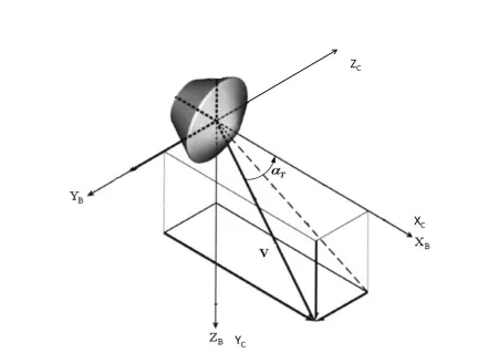
It is necessary that the telemetry data be transformed into a body coordinate

system (see Fig. 3.1), since the aerodynamic forces and moments are referenced to a body

coordinate system. The origin of both the body axis frame and cruise frame is at the

center of mass, the XB axis is through the axis of symmetry, the YB axis is perpendicular

to the x axis and the ZB axis makes a right hand orthogonal system9,3. The V vector in

Fig. 3.1 is the atmosphere relative velocity vector and the angle between the atmosphere

relative velocity vector and the x-axis is the total angle of attack.

Figure 3.1 Body-axis (XB, YB, ZB) and cruise-axis (XC, YC, ZC) coordinate systems.

The location of the IMU frame was measured in relationship to the entry vehicle

(23)

coordinate system is not time dependent, thus, the transformation is accomplished once

for the entire data sets with the quaternion in Table 3.1. MER A and MER B had two

IMUs (one on the Rover and the other on the disposable backshell) that collected data

during entry and both are included in the table.

Table 3.1 Body coordinate system to IMU frame quaternion.

q1 q2 q3 q4

MER A Rover -0.00030 -0.70709 -0.70712 0.00081 MER A Backshell 0.18247 0.31915 0.80510 0.46547 MER B Rover -0.00061 -0.70702 -0.70719 0.00001 MER B Backshell 0.18661 0.32252 0.80405 0.46331 Phoenix 0.67642 0.48052 0.51795 0.20806

It was desired that all three missions use a common time system such that

comparisons between the flight data from each mission can be made. The time reference

point for all three vehicles was based an entry interface altitude, which occurred at an

altitude of 125 km. Mission operations and mission designers commonly use this

reference. At this altitude, the atmospheric drag is typically lower than the accelerometer

sensitivity threshold.

The raw telemetry data was available for Phoenix for the length of the entry, but

for MER A, and MER B the telemetry data was available only after 90 seconds after

entry interface. The telemetry data available for MER A, and MER B before 90 seconds

were processed by the onboard navigation computer and as such, is currently in the body

axis frame. The angular rates for MER A, and MER B before 90 seconds were derived

from the quaternion and more details are given in the proceeding section.

All telemetry data sets were processed for the trajectory from entry interface to

(24)

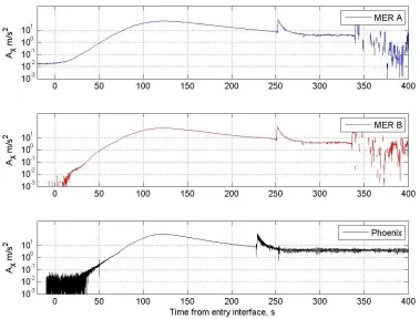
this analysis stops at parachute deployment. Fig. 3.2 y-axis shows the positive body

x-axis accelerations on a log scale as a function of linear time for MER A, MER B, and

Phoenix; top, middle and bottom figures respectively. The parachute deployment

occurred near 250 seconds from entry interface for both MER A, and MER B and near

228 seconds from entry interface for Phoenix as shown in Fig. 3.2. In Fig. 3.2, the

parachute deployment appears as the largest peak in acceleration, and an abrupt jump in

acceleration precedes the peak.

At entry interface, the accelerations due to the atmosphere drag are near the

sensitivity limits of the IMU and are denoted in Fig. 3.2 with very small acceleration

levels accompanied with relatively large oscillation in acceleration. The analysis of the

flight data started after a steady increase in acceleration was observed in Fig. 3.2. The

steady increase in acceleration was the result of higher atmospheric drag and indicated

that the atmospheric drag is above the accelerometer sensitivity threshold. The

accelerometer sensitivity threshold is mission dependent, as seen in Fig 3.2. The time of

the accelerometer sensitivity threshold occurred at about 10 seconds from entry interface

for both MER A and MER B missions and about 35 seconds from entry interface for

Phoenix. The times for accelerometer sensitivity threshold and parachute deployment set

the time domain for the MEVAD validation. That is, only trajectory data after the

accelerometer sensitivity threshold and before parachute deployment were used for the

comparison and subsequent validation. The time domains used for the comparison and

validation for MER A, and MER B are from 10 to 250 seconds from entry interface and

(25)

Figure 3.2 Accelerations along the body x-axis for MER A, MER B, and Phoenix.

The final part of step one was to define an inertial coordinate system where the

equations of motion were integrated. The inertial coordinate system selected was the

Planet Inertial Coordinated System (PICS), which placed the origin at the center of mass

of the planet and the fundamental plane along the equator. The x-axis is along the Mars

vernal equinox, and the z-axis is along the rotational axis of the planet with positive

direction in the direction of the north pole9. The processing of the accelerations and

angular rates is discussed in section 3.2, and is performed in the body axes coordinate

(26)

3.2 Step two.

Step two goal was to process the telemetry data in order to make adjustments in

the measured values and in order to prepare the telemetry data for integration of the

equation of motion in the PICS. Measurement adjustments are needed for a variety of

reasons, such as, the digitizing process, misalignments, sensor biases and sensor noise.

Part of the data processing also included determining angular accelerations, correcting for

center of mass offset of the accelerometers and transforming the telemetry data from the

body axis coordinate system to PICS. At the end of data processing, all steps are

completed such that the integration of the equation of motion in PICS can be

accomplished.

The telemetry data was processed first to reduce noise from the sensors, which

involved filtering the telemetry data. There were two methods for filtering telemetry data

utilized in the validation process, namely batch filtering and pass filtering. The

low-pass filtering was needed because of the separation in sampling frequencies between

MER and Phoenix missions. Phoenix had a sampling frequency of 200 Hz where MER

A, and MER B had a sampling frequency of 8 Hz. The higher frequency signals in

Phoenix telemetry data introduced unwanted noise from the over sampling. The removal

of the unwanted high frequency signals in Phoenix telemetry data was completed in such

a way as to maintain frequencies similar to the frequencies recorded by the MER

sampling rate. The low pass filter, which removed the unwanted high frequency signals,

uses a cut off frequency to remove higher frequencies10. The cut off frequencies utilized

(27)

The batch filtering method removed noise by fitting a second order polynomial to

a batch of data. A batch of data, i.e. number of data points over a time period, ranged

from 7 to 901 data points as required for a specific data set, discussed later in this section.

The measured angular rates for each mission are used to correct the accelerations

for center of mass offset. In order to accomplish these corrections, angular accelerations

are needed. Angular accelerations were determined from numerically differentiating the

measured angular rates. As result of the angular rates being used to correct the

accelerations and to determine the angular accelerations, the angular rates are processed

first. It is vital that the angular rates be processed correctly, as any error in the angular

rates will propagate through to the calculations of aerodynamic coefficients discussed in

section 7.

The measured angular rates were recorded for Phoenix throughout entry and for

MER A, and MER B starting at 90 seconds from entry interface to landing. The angular

rates after 90 seconds from entry interface for MER A, and MER B are used in

combination with the angular rates determined from the quaternion before 90 seconds

from entry interface. The angular rates for MER A, and MER B before 90 seconds from

entry interface were determined from the quaternion using the following,

(3.1)

where ωx, ωy, and ωz, are the components of the angular rates, q is the quaternion and is

(28)

Determining the angular rate from the quaternion required that a derivative of the

quaternion be determined which can potentially create additional noise in the rate data.

These numerical differentiating errors could affect the angular rates significantly.

Fortunately, from entry to 90 seconds from entry interface there was not a significant

change in angular rates.

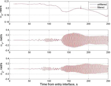
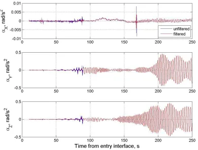
The angular rates along the x, y, and z axes for MER A are shown in Fig. 3.3 top,

middle, and bottom respectively with the blue line being the unfiltered angular rates and

the red being the filtered angular rates. The angular rate about the x-axis shows an

unexpected change around 120 seconds from entry interface, which will be discussed in

the section 7. The change in angular rate in the x-axis is unexplained because the entry

vehicle is supposed to be axisymmetric and therefore should not have a rolling moment,

Cl, which would cause a change in angular rate. The largest difference between the

filtered and unfiltered angular rates was a spike in the x-axis around 170 seconds from

entry interface.

The angular rates from 90 seconds after entry interface to parachute deployment

were filtered by using a second order least square fit over 7 data points. Several batch

sizes were tested to determine the optimal batch size. The criterion for selecting the

optimal batch size was the sum of residual from the unfiltered and filtered data sets that

(29)

Figure 3.3 MER A angular rates in body coordinate system.

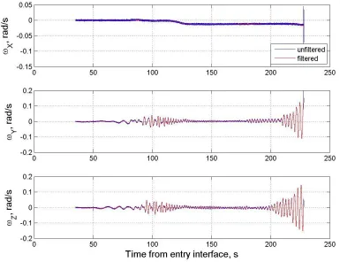
MER B angular rates are presented in Fig. 3.4. The results for the filtered angular

rates are similar to MER A. The largest difference after the angular rates were filtered

occurred in the x-axis around 170 seconds from entry interface. The angular rates from

90 seconds after entry interface to parachute deployment were filtered by using a second

order least squares fit over seven data points, basically using the same process as MER A.

Like MER A, the x-axis has an unexpected change in angular rate near 140 seconds from

(30)

Figure 3.4 MER B angular rates in body coordinate system.

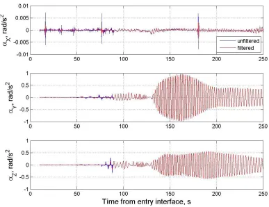
Phoenix angular rates are presented in Fig. 3.5. The unfiltered angular rates for

Phoenix (indicated by a blue curve) contained significantly higher noise levels compared

to MER A, and MER B, as seen in Figs. 3.3 and 3.4. (Note: the blue curve in the Phoenix

figure is more dominant than on either MER A or MER B figures). This noise is most

likely due to a combination of digitization and over sampling. The y and z axes angular

rate presents significantly smaller amplitude compared to the y and z axes MER A, and

MER B. The amplitude difference in angular rates in the y and z axes is most likely the

result of the torque from the thermal blanket for MER A, and MER B12. Phoenix

(31)

130 seconds from entry interface. A low pass filter with a cutoff frequency of 17 Hz was

used for filtering the angular rates from Phoenix.

Figure 3.5 Phoenix angular rate components in cruise coordinate system.

With the angular rates accomplished, the next process was to determine the

body-axis to inertial quaternion and angular accelerations for each entry vehicle. The

quaternion is needed to transform the telemetry data from the body axis coordinate

system into the PICS. The angular accelerations were needed to correct for center of mass

offset in the accelerations and for calculating the aerodynamic torque applied to the

(32)

The angular accelerations were determined by subtracting each adjacent filtered

angular rate and dividing by the time difference. The angular accelerations were then

filtered in a similarly manner as the angular rates. Again, it is necessary to take the

derivative of digital data, which could add noise to the data. The noisy signals are most

clearly visible in the angular accelerations before 90 seconds from entry interface for

MER A, and MER B shown in Figs.3.6 and 3.7, where the angular accelerations are the

results of two derivatives; one to obtain the angular rate from the quaternion, and the

other to get the angular acceleration from the angular rates.

MER A angular accelerations for the x, y, and z axes are presented in Fig. 3.6 top,

middle, and bottom respectively. The blue lines are the unfiltered angular accelerations

and the red are filtered angular accelerations, which were filtered with a second order

polynomial over seven data points. The increase in angular acceleration and

non-symmetric values along the x-axis between 110 and 150 seconds from entry interface

indicates that a torque was applied to the entry vehicle. The increase in noise level on the

angular accelerations from entry to 90 seconds from entry interface was the result of two

(33)

Figure 3.6 MER A angular accelerations in body coordinate system.

MER B angular accelerations are shown in Fig. 3.7. The accelerations were

filtered with a second order polynomial over seven data points. The angular acceleration

about the x-axis is symmetric with the exception of a 7 second region near 130 seconds

(34)

Figure 3.7 MER B angular accelerations in body coordinate system.

The angular accelerations for Phoenix are shown in Fig. 3.8 and were filtered with

a low pass filter with a cutoff frequency of 15 Hz. The x-axis angular acceleration

produced a slight decrease between 80 and 130 seconds from entry interface. The

increase in angular acceleration amplitude after 200 seconds from entry interface is the

(35)

Figure 3.8 Phoenix angular accelerations in body coordinate system.

As mentioned earlier, a quaternion was utilized to transform the acceleration data

from the body coordinate system to PICS. The body coordinate system changes in

relation to PICS throughout entry and thus is time dependent. The quaternion for MER A

and MER B (shown in appendix H) transfers the telemetry data from body coordinate

system to Earth J2000 coordinate system, which a direction cosine matrix (DCM) (shown

in table 3.2 and 3.3) is used to transfer to the PICS. The Earth J2000 coordinate system is

based on Earth mean equator and equinox of J2000 and is changing with respect to PICS,

(36)

coordinate system to PICS transformation was assumed to be a fixed rotation9. For the

Phoenix data set, the cruise frame coordinate system to PICS is directly available.

Table 3.2 MER A PICS to Earth J2000 DCM

0.673307067 -0.589579915 0.446153693 0.739362965 0.53690588 -0.406293591 0 0.603429863 0.797416077

Table 3.3 MER B PICS to Earth J2000 DCM

0.6733078544 -0.589579070 0.446153620 0.739362247 0.536906259 -0.406294394 0 0.603430350 0.797415708

The JPL navigation team estimated the sun unit vector of MER A and MER B at

entry interface. The sun unit vector is in the direction of the sun from the entry vehicle in

Earth J2000 coordinate system at entry interface9. It is necessary to rotate about the sun

unit vector to achieve reasonable landing position and velocity. The proper rotational

angle was determined for MER A, and MER B by using the landing conditions and

parachute conditions to determine a feasible match. The resulting rotational angle about

the sun vector was adjusted to -0.5 and -0.75 degrees for MER A, and MER B

respectively. Changing the rotational angle about the sun unit vector by more than 2

degrees caused trajectory parachute and landing conditions to be unrealistic. Small angle

rotations about the sun vector have a large impact on parachute deployment conditions

and a large impact on the trajectory angle of attack after the second hypersonic

instability.

The quaternion was calculated for Phoenix using an initial condition provided by

(37)

(3.2)

where q is the quaternion, is the derivative of the quaternion and ω is the filtered

angular rates.

The last part of the data processing section focuses on the accelerations. The

accelerations were first filtered then transformed into the PICS utilizing the body axis

coordinate system to PICS quaternion. The basic filtering of the accelerations utilized the

same processes as the angular rates; however, in addition biases were determined since

accelerations data was recorded before entry interface. The accelerations unlike the

angular rates had two special issues, the first was to correct for a center of mass offset

and the second was correct for a misalignment.

The accelerations like the angular rates were measured by the IMUs. However,

the accelerations values from the IMUs are not based at the center of mass of the entry

vehicle, required by the equation of motions. The measured accelerations include the

accelerations at the center of mass and a rotational acceleration component, which it is

necessary to remove. The removal of the rotational component in the acceleration was

accomplished using,

( 3.3)

where AIMU is the acceleration value from the IMU, is the angular acceleration, ω is the

angular rate, Rcti is the distance from the IMU to the center of mass of the entry vehicle

which is given in component form in Table 3.4, and Acom is the acceleration at the

(38)

Table 3.4 Distance Components from the IMU to COM in the Body-Axis Frame.

X (m) Y (m) Z (m)

MER A Rover -0.1757 0.2328 0.043 MER A Backshell -0.4454 -0.2497 -0.5299 MER B Rover -0.1757 0.2329 0.0439 MER B Backshell -0.445 -0.2499 -0.5296 Phoenix -0.2187 0.5197 0.2284

After the accelerations were corrected for the center of mass offset, the biases

were determined with acceleration data before entry interface. Before entry interface, the

entry vehicle will have little detectable acceleration as atmospheric drag is well below the

acceleration sensitivity threshold discussed earlier. This period before entry interface

allows for an opportunity to determine the bias for the accelerometers. The integrated

velocity values over several seconds before entry interface were fit with a first order

polynomial for all three entry vehicles. The bias value for an accelerometer was the slope

in the first order polynomial and bias values presented for each mission in Table 3.5.

Table 3.5 Biases by mission.

x (m/s2₎ _{y (m/s}2₎ _{z (m/s}2₎

MER A 1.36E-08 -2.11E-07 -3.77E-07

MER B 5.32E-05 2.36E-07 2.36E-05

Phoenix -3.85E-04 2.10E-04 4.21E-04

With the acceleration corrected to the center of mass and biases removed, the

accelerations from the rover and backshell IMUs are compared for MER A. Shown in

Ref. 11, the accelerations from the rover and backshell disagree. MER B rover and

backshell corrected acceleration showed similar results. The disagreement in

accelerations indicates that one or both of the IMUs were misaligned. A misalignment in

(39)

coordinate system to be measured in the y and z axes of body coordinate system. The

portion of x-axis accelerations measured in y and z axes was determined by projecting the

x-axis acceleration onto the accelerations of the y and z axes of the body coordinate

system in a linear least squares fit. The slope of the linear least squares fit was interpreted

as the misalignment in the IMU11. The acceleration data used in the linear least squares

projection was limited to two regions, the first one being entry to 10 second from entry

interface and the second one from 140 to 250 seconds from entry interface. The resulting

misalignments angles are used to correct MER A, and MER B rover IMU accelerations

and are presented in Table 3.6. Shown in Ref. 11, after the IMU misalignment correction

the acceleration data from both rover and backshell IMUs agree well for both MER A,

and MER B. The misalignment angles determined for this validation are within 0.005

degrees of the misalignment angles determined from Ref. 11.

Table 3.6 Misalignments in the rover IMU accelerations.

y (deg.) z (deg.)

MER A 0.0418 -0.0362

MER B 0.0363 -0.0462

Like the MER A and MER B angular rates, the accelerations for are split before

and after 90 second from entry interface. The onboard navigational computer processed

the accelerations before 90 seconds from entry interface. The accelerations after 90

seconds from entry interface were filtered using a second order polynomial over a batch

of data. The two acceleration data set time segments were combined into one data set for

purpose of this validation.

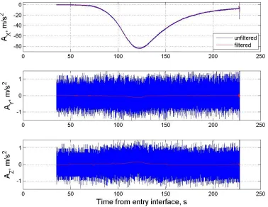
The unfiltered and filtered/corrected acceleration data sets from the MER A rover

(40)

been corrected for the misalignment. The misalignment correction to the non-axial forces

produces the largest change during the instability regions. The misalignment correction in

the acceleration in the y-axis body coordinate system shown in the middle panel of Fig.

3.9 acts as a bias correction during the first and second instability resigns. The

misalignment correction in acceleration along the z-axis shown in the bottom panel of

Fig. 3.9 shifts the acceleration by less than 0.02 m/s2. The MER A acceleration data from

90 seconds from entry interface to parachute deployment was filtered using a second

order least squares fit over seven data points.

(41)

MER B x, y, and z axes accelerations in the body coordinate system are shown in

Fig. 3.10 top, middle, and bottom respectively. The accelerations measured from the

backshell IMU were used from entry to 90 seconds from entry interface and for the

remainder of the acceleration data set, the rover IMU accelerations were used. The rover

accelerations were fit with a second order least squares fit over seven data points. The

misalignment correction shifted the acceleration less than 0.004 m/s2 during the

instability regions.

Figure 3.10 MER B accelerations in body coordinate system.

Phoenix x, y, and z axis accelerations in cruise frame are shown in Fig. 3.11 top,

(42)

large amount of noise. Two filters are used to remove noise from the Phoenix

accelerations. A low pass filter with a cut off frequency of 15 Hz was used first to remove

the high frequency noise. The low frequency noise in the accelerations was decreased by

fitting a second order polynomial over 901 data points. The second filter was utilized due

to concerns that a lower cut off frequency for the low pass filter would remove parts of

the acceleration signal.

Figure 3.11 Phoenix acceleration components in cruise coordinate system.

3.3 Step three.

The final step was to integrate the equations of motion in the PICS. The equations

(43)

equation of motion required the initial conditions and the telemetry data, which was

transformed into PICS. The initial conditions for all three missions came from the

onboard navigation computer at entry interface and are given in Table 3.7.

Table 3.7 Initial conditions for Mars entry missions in PICS.

X (m) Y (m) Z (m) Vx (m/s) Vy (m/s) Vz (m/s)

MER A -2,833,658 -1,800,899 -1,064,442 3,522 -4,166 1,383

MER B -3,128,460 -1,608,596 -176,209 3,535 -4,445 469

Phoenix 1,060,216 -645,718 3,296,296 1,465 5,350 -771

The equations of motion for the entry vehicle in PICS are defined as,

(3.4)

The gravitation term is defined in PICS by differentiating the gravitational potential

function. The gravitational model used in the integration process contains up to the

second zonal harmonic, a portion of which is shown as,

(3.5)

where x, y, and z are the corresponding location in PICS, r was the magnitude of the

position vector, J2 is the second zonal harmonic of Mars, RMars is the equatorial radius of

Mars and µ is the gravitation parameter of Mars14.

Areodetic altitude was determined from position and was used for interpolation of

the atmospheric models discussed in the next section. The areodetic altitudes for all three

missions were determined utilizing the methods defined in Ref. 15. The solution for the

(44)

oblate spheroid15. The resulting areodetic altitudes by time from entry interface are

present in top of Fig. 3.12 with MER A in blue, MER B in red, and Phoenix in black.

The velocity determined from the integration of the equations of motion was the

inertial velocity in the PICS frame and as such does not include the rotation of the

Martian atmosphere. In addition, the MEVAD requires angle of attack, sideslip angle,

and Mach number for interpolation, which require the atmospheric relative velocity. The

atmospheric relative velocity was determined by assuming a rigid rotating atmosphere

using,

(3.6)

where Vx, Vy, and Vz are the atmospheric relative velocity components in PICS, VintX,

VintY, and VintZ are the velocities in PICS from the integration of the equation of motions,

and ωMars is the angular rotation rate of Mars.

The magnitude of velocity of the entry vehicle, corrected for the rigid rotating

atmosphere, is present in bottom of Fig. 3.12. MER A and MER B entered the

atmosphere of Mars with a velocity around 5.3 km/s, where Phoenix had a slightly higher

velocity of around 5.5 km/s. All three entry vehicles had a velocity between 0.3 and 0.45

km/s at parachute deployment with Phoenix parachute deployment occurred earliest near

(45)

Figure 3.12 Areodetic altitude and atmospheric relative velocity of the MER A,

MER B, and Phoenix entry vehicles.

The atmospheric relative velocity was transferred from PICS into to the body

coordinate system using the quaternion from section 3.2. The atmospheric relative

velocity (assuming no winds) was utilized to determine the total angle of attack, angle of

attack, and sideslip angle from,

(46)

_(3.8)

(3.9)

The total angle of attack for MER A, MER B, and Phoenix is presented in Fig.

3.17 top, middle, and bottom respectively. The instability regions are clearly visible in

MER A, and Phoenix. The first and second instabilities occurred for MER A and Phoenix

near 75 and 125 seconds from entry interface. The first instability is not clearly visible for

MER B; however, there was some question before launch if MER A, and MER B would

go through the first instability16. The second instability for MER B occurred near 125

seconds from entry interface.

(47)

4. Atmospheric models.

The comparison between MEVAD and flight aerodynamic coefficients require the

trajectory results from integration of the equations of motion and atmospheric state

properties. The atmospheric state properties, namely pressure and density, are used to

determine Mach numbers, and Knudsen numbers in the interpolation of MEVAD.

Further, density is also needed in the calculation of all the flight derived aerodynamic

coefficients. Lacking atmospheric measurement information during the entries introduce

special challenges in obtaining flight aerodynamic coefficients. To help mitigate the lack

of atmosphere measurements, and to limit the dependence of the analysis of unknown

atmosphere properties, two independent approaches for determining density have been

developed. The first method for determining the atmospheric properties was simply using

the preflight models for MER A, MER B, and Phoenix. The preflight atmosphere models

main focus was to predict winds near the surface17,19. The second method employed a

well-documented procedure utilized by earlier researchers, of using the axial coefficient,

CA along with the axial measurement acceleration to obtain a flight extracted density.

From density and the gravity model, the pressure is calculated from the hydrostatic

equation, discussed later.

The purpose for using two independent atmosphere models is to consider flight

coefficient data during instances when both models produce coefficients with small

differences. The densities from the two methods in determining coefficients from

MEVAD are displayed and discussed in section 5. The two atmosphere models are also

(48)

4.1 Flight extracted model.

The flight extracted model calculated density using,

(4.1)

In the density equation, CA is a function of total angle of attack, t and Mach number, M

and is a transcendental equation because density appears on both sides of the equation

and cannot be separated algebraically. To solve the CA equation requires an iterative

process. This is accomplished by assuming an initial estimate of CA and subsequently

iterating with the database. That is, with the new CA, the cycle repeats until the change in

density decreased to 0.001 percent of the previous density value. The trajectory

reconstructed total angle of attack, t and the corresponding aerodynamic database for

that particular mission were used when acquiring the CA . The Mach number calculation

is shown subsequently.

In conjunction with the density being calculated from equation 4.1, the pressure

was calculated by integrating the hydrostatic equation as such,

(4.2)

The flight extracted atmosphere approach started at entry interface where the atmospheric

pressure was near zero. For the initial pressure, zero was assumed.

With these properties determined, Knudsen numbers and Mach numbers were

simultaneously calculated. The resulting Mach number and Knudsen numbers are shown

(49)

The atmosphere properties of importance to the database application are Mach

number and Knudsen number. The Mach number calculations follows,

(4.3)

where the V is the atmospheric relative velocity and s is the speed of sound. The speed

of sound was calculated using,

(4.4)

The Knudsen number is defined as,

(4.5)

where λd is the mean free path and Lreff is the reference lengths for MER and Phoenix

entry vehicles, which were 2.65 meters16,3. The mean free path is,

(4.6)

4.2 Atmosphere models effect on MEVAD inputs.

The two atmosphere dependent inputs to the MEVAD are Mach number and

Knudsen number. It is necessary to show the difference that the atmosphere models have

on the inputs to the database. This is discussed next.

The atmospheric proprieties determined from both models introduced in this

section generate two values of Knudsen numbers and two values of Mach numbers. The

two resulting Mach and Knudsen numbers for MER A are shown in Fig. 4.1 top and

bottom respectively. The solid blue line is the Mach numbers and Knudsen numbers

determined utilizing the flight extracted atmospheric model and the red dotted line are the

(50)

model. The vertical dotted blue line is the transition line from transitional flow to

continuum flow. The Mach numbers from the two atmospheric models agree with the

exception of the first 30 seconds from entry interface. This difference occurs when the

flow regime is transitional flow so Mach numbers were not used for interpolation for this

period. The greatest difference in Mach number, where Mach number was used for

interpolation into the aerodynamic database, was less than 1.7 and it occurred near 95

seconds after entry interface. The largest difference in Knudsen number, which was less

than 50 percent, occurred at entry interface then decreased until 40 seconds from entry

interface. This large difference in Knudsen number will require a comparison in the

resulting interpolated coefficients from MEVAD for both methods of determining

(51)

Figure 4.1 MER A Mach and Knudsen numbers for flight exacted and preflight

atmospheres.

MER B resulting Mach and Knudsen numbers are shown in Fig. 4.2 top and

bottom respectively. From entry interface to 25 seconds from entry interface the flight

extracted model suffered from small accelerations, which caused large fluctuation in

density and resulted in the signal issues in Mach and Knudsen numbers. The greatest

difference between the flight extracted and preflight models for Mach number occurred

before 40 seconds from entry interface, however, this was in the transitional flow

regimes. The largest difference in Mach numbers where the Mach numbers were used for

(52)

125 seconds from entry interface to parachute deployment there was not a significant

difference between atmospheric models for Mach numbers. MER B Knudsen numbers

models agree very well with the exception of from entry interface to around 40 seconds

from entry interface, which produced a difference less than 50 percent. Again this

difference in Knudsen will require a comparison of the resulting coefficients from

MEVAD shown later in this section.

Figure 4.2 MER B Mach and Knudsen numbers for flight extracted and

(53)

Mach and Knudsen number results for Phoenix are shown in Fig. 4.3. The Mach

numbers from both atmospheric models agrees well throughout entry. The maximum

difference in Mach numbers between the atmospheric models after 80 seconds from entry

interface was less than 1.7 and it occurred near 110 seconds from entry interface. The

Knudsen number comparisons shows a constant, but relatively small, difference between

the preflight and flight extracted atmospheric models with the preflight model producing

higher Knudsen number throughout the entry. The difference in the resulting coefficients

from the interpolation of MEVAD utilizing both methods of determining atmospheric

(54)

Figure 4.3 Phoenix Mach and Knudsen numbers for flight exacted and

preflight atmospheres.

5. Atmosphere effects on MEVAD coefficients.

It is important to understand the effects that the two atmosphere models have in

term of the aerodynamic coefficients. To accomplish this goal, the Mach number and

Knudsen number (the MEVAD input quantities) time histories using the preceding

equations for each of the three entry mission have been performed. The results from the

preceding equation (using CA, measured acceleration, and trajectory reconstruction

results) are referred to as “flight” Mach number and Knudsen number. In addition, the

same calculations are made substituting the three preflight model atmosphere properties

and are labeled “preflight” Mach number and Knudsen number. The difference results

from both calculations are presented and discussed next.

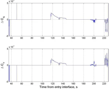
The differences in the interpolated coefficients from MEVAD for MER A force

and moment coefficients utilizing both atmosphere models of determining atmospheric

properties are presented in Figs. in 5.1, and 5.2. The difference in the coefficients near

125 seconds from entry interface occurred during the second hypersonic instability,

which the coefficients from MEVAD in this region are very sensitive to density. The

difference in density from the two methods appeared as an oscillation from 200 seconds

from entry interface to parachute deployment. The uncertainties for in the MEVAD for

MER (given in the Appendix D) is 0.01 for the force coefficients. Thus, the largest

coefficient difference due to the atmosphere models is about 4 percent of the database

(55)

for the hypersonic and supersonic flight regimes respectively9. Thus, the differences in

the moment coefficients are less than of 3 percent of the MEVAD uncertainty.

Figure 5.1 MER A database force coefficient differences using two atmospheric

(56)

Figure 5.2 MER A database moment coefficient differences using two

atmospheric models.

The differences in the interpolated force and moment coefficients from MEVAD

for MER B utilizing both methods for determining atmospheric properties are shown in

Figs. 5.3 and 5.4. The difference near 10 seconds from entry comes from the fluctuations

in acceleration used to determine the flight extracted atmospheric model. The oscillation

near 175 seconds from entry interface to parachute deployment was the result of a

difference in density. The differences from MEVAD are larger for MER B than for MER

(57)

Figure 5.3 MER B database force coefficient differences using two atmospheric

(58)

Figure 5.4 MER B database moment coefficient differences using two

The differences in the interpolated force and moment coefficients from MEVAD

for Phoenix utilizing both methods for determining atmospheric properties are shown in

Figs. 5.5 and 5.6. The differences near 35 second from entry interface was the result of

acceleration fluctuations from the flight extracted atmospheric model, and the differences

around 120 seconds from entry interface were the result of MEVAD sensitive to density

during the second hypersonic instability. The uncertainties from MEVAD for Phoenix for

CN and CY are 0.01 and 0.08 respectively. The moment coefficient uncertainties for Cm

(59)

supersonic regime3. The differences inthecoefficients are less than 8 percent of the

uncertainty of MEVAD for Phoenix.

Figure 5.5 Phoenix force database force coefficient differences using two

(60)

Figure 5.6 Phoenix database moment coefficient differences using two

The differences in the interpolated coefficients from MEVAD for the two

methods of determining atmospheric properties are less than 10 percent uncertainty of the

MEVAD force and moment coefficient uncertainty for all three entries. The 10 percent of

uncertainty of MEVAD results indicate that the atmosphere models produce the same

force and moment coefficients within 10 percent uncertainty of the database. This is good

(61)

6. Density effects on flight derived aerodynamic coefficients.

It has been established that using either atmosphere models (“flight” or

“preflight”) produce equivalent aerodynamic coefficient (within an acceptable tolerance,

10 percent) from the database. In this section, the flight coefficient using both atmosphere

models are generated. The results from this analysis use the same nomenclature as the

preceding section. That is, “flight” is used when flight derived atmosphere properties are

used and “preflight” is used when the atmosphere models are used. The flight and

preflight derived aerodynamic coefficients are the CN, CY, Cm, Cn, and Cl.

The flight derived aerodynamic coefficients were calculated using,

(6.1)

(6.2)

(6.3)

(6.4)

(6.5)

where Ay, and Az are accelerations in the y and z axes of the body coordinate system. Mx,

My, and Mz are the moments about the x, y, and z axes of the body coordinate system

(62)

(6.6)

(6.7)

(6.8)

The moments of inertia and mass for each entry vehicle used to calculate the flight

derived aerodynamic coefficients are presented in Table 6.1.

Table 6.1 Moments of inertia and mass.

Ixx

(Kgm2₎ _(KgmIyy 2₎ _(KgmIzz 2₎ _(KgmIxy 2₎ _(KgmIxz 2₎ _(KgmIyz 2₎ Mass _(Kg) MER A 365.605 278.6485 272.0971 -0.03154 -0.01674 -0.64161 811.7 MER B 276.424 264.923 368.0042 -2.22856 0.010403 -0.01925 811.7 Phoenix 285.552 179.665 201.223 0.0002 0.14 3.997 602

An aerodynamic coefficient sample from each of the three entry missions flight

derived coefficients using the two atmosphere models is presented. The remaining flight

derived coefficients determined with the two atmosphere models are not shown here, but

yield similar conclusions.

MER A flight derived CN from the flight extracted and preflight atmospheric

models are shown in the top panel of Fig. 6.1 blue and red respectively. The percent

difference between the CN from the two atmospheric models, based upon the uncertainty

from MEVAD, is presented in the bottom panel of Fig. 6.1. The two atmospheric models

come into agreement near 50 seconds from entry interface. Prior to 50 seconds, the

differences are due to density differences. From 50 seconds from entry interface to

parachute deployment the difference in CN from the two methods of determining

atmospheric properties is small, less than of 0.0025, which resulted in a percent

Aerodynamic Validation using MER and Phoenix Entry Flight Data.

Abstract

Data

Biography

Acknowledgements

Table of Contents

List of Figures

List of Tables

Nomenclature

1.

Introduction.

2.

Mars Entry Vehicle Aerodynamic Database.

3.

Entry trajectory reconstruction.

4.

Atmospheric models.

5.

Atmosphere effects on MEVAD coefficients.

6.

Density effects on flight derived aerodynamic coefficients.