Regression and ANN models for estimating minimum value of machining performance

(1)

Regression and ANN models for estimating minimum value

of machining performance

Azlan Mohd Zain

a,⇑

, Habibollah Haron

a

, Sultan Noman Qasem

a

, Saﬁan Sharif

b

a

Soft Computing Research Group, Faculty of Computer Science and Information Systems, Universiti Teknologi Malaysia, 81310 UTM Skudai, Johor, Malaysia

b

Department of Manufacturing and Industrial Engineering, Faculty of Mechanical Engineering, Universiti Teknologi Malaysia, 81310 UTM Skudai, Johor, Malaysia

a r t i c l e

i n f o

Article history:

Received 1 September 2010

Received in revised form 27 August 2011 Accepted 1 September 2011

Available online 8 September 2011

Keywords: Modeling Regression ANN

Minimum surface roughness End milling

a b s t r a c t

Surface roughness is one of the most common performance measurements in machining process and an effective parameter in representing the quality of machined surface. The minimization of the machining performance measurement such as surface roughness (Ra) must be formulated in the standard mathematical model. To predict the minimum Ravalue, the process of modeling is taken in this study. The developed model deals with real experimental data of theRain the end milling machining process. Two modeling approaches, regression and Artiﬁcial Neural Network (ANN), are applied to predict the min-imumRavalue. The results show that regression and ANN models have reduced the min-imumRavalue of real experimental data by about 1.57% and 1.05%, respectively.

1. Introduction

The developed model for the machining process is a mathematical equation that shows the relationship between two parameters, process parameters (decision variables) and machining performance (responses). Fundamentally, models can be divided into three categories which are experimental models, analytical models and Artiﬁcial Intelligent (AI) based mod-els. Experimental and analytical models can be developed by using conventional approaches such as Regression technique. While, AI based models are developed using non-conventional approaches such as Artiﬁcial Neural Network (ANN).

The difference between the regression model and ANN lies mainly in the nonlinear regions[1]. ANNs can be used as an

effective and an alternative method for the experimental studies whose the mathematical model cannot be formed [2].

Regression technique may work well for machining process modeling as reported by many previous studies. A mathematical model was developed using regression model for surface roughness in wire electrical discharge machining, and it was found that the developed model showed high prediction accuracy within the experimental region. The maximum prediction error

of the model was less than 7%, and the average percentage error of prediction was less than 3%[3]. The regression model

showed a slightly better performance compared to the ANN model for modeling surface roughness in abrasive waterjet

machining[4]. However, regression model may not precisely described the underlying non linear complex relationship

between decision variables and responses[5]. ANN and Regression models are used to model the surface roughness and tool

wear machining performance in hard turning machining [6]. As a result, the ANN models provided better prediction

capabilities because they generally offer the ability to model more complex nonlinearities and interactions than linear and exponential regression models can offer. ANN model follows the machining experimental data much more closely than

that from regression model[1].

⇑Corresponding author. Tel.: +60 7 5532088; fax: +60 7 5565044/5574908. E-mail addresses:[email protected],[email protected](A.M. Zain).

Contents lists available atSciVerse ScienceDirect

Applied Mathematical Modelling

(2)

The literatures show that surface roughness (Ra) is one of the performance measures studied mostly by researcher in

modeling problem. Some recent studies deal with ANN for modeling surface roughness in various machining operations such

as wire electrical discharge machining[7,8], turning[9–12], and milling[13–18]. With Regression and ANN as the considered

modeling techniques, the objective of this paper is to study the prediction result for surface roughness performance measure in end milling machining operation. ANN model gave a high accuracy rate (96–99%) for predicting machining performance

(surface roughness) in end milling operation compared to the result obtained from regression model[19]. It was reported

that the minimization ofRamachining performance in end milling involving radial rake angle process parameter is still

lack-ing, in particular when dealing with titanium alloys. As such optimization of the cutting conditions, which include radial rake

angle, combined with cutting speed and feed, for theRain end milling of Ti–6Al–4V can be considered as a new contribution

to the machining research.

2. Modeling of surface roughness

Modeling is described as a scientiﬁc way to study the behaviors involved in the process. Modeling of machining processes is important for providing the basis mathematical model for the formulation of the objective function. A model developed for machining process is the relationship between two variables which are decision variable and response variable in terms of

mathematical equations. Therefore, the minimization of theRamust be formulated in the standard mathematical model.

Normally, the model of the predictedRacan be expressed as in Eq.(1):

Ra¼k

Yn

i¼1

cei

i: ð1Þ

Eq.(1)can also be written as follows:

Ra¼kc

e1 1c

e2 2c

e3 3 c

en

n; ð2Þ

whereRais the predicted surface roughness (respond variable),c1 cnis the cutting conditions (decision variables), andk,

e1,e2,e3,. . .,enare the model parameters to be estimated using the experimental data.

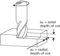
In the milling process, material is removed from the workpiece by a rotating cutter. The milling process can be classiﬁed into two parts; peripheral milling and face milling. Peripheral milling generates a surface parallel to the spindle rotation, while face milling generates a surface normal to the spindle rotation. End milling is a type of face milling, and is used for

facing, proﬁling and slotting processes.Fig. 1shows an illustration of interaction between cutting tool and workpiece for

removing material in the end milling process.

In the end milling process, the surface can be generated by two methods; up milling and down milling. Up milling is also called conventional milling; the cutter rotates against the direction of feed of the workpiece. Down milling is also called

climb milling; the rotation is in the same direction as the feed. These processes are illustrated inFig. 2.

A machining experiment was conducted based on the down milling process[20]. A mathematical model of the predicted

Rais expressed in Eq.(3)

Ra¼k

v

e1_fe2

_c

e3_; _ð₃_Þ

whereRais the predicted surface roughness in

l

m,

v

is the cutting speed in m/min,fis the feed rate in mm/tooth,

c

is the

radial rake angle in°, andk,e1,e2ande3are the model parameters to be estimated using the experimental data.

2.1. Regression modeling

To develop the regression model for estimating theRavalue, the mathematical model given in Eq.(3)is linearized by

per-forming a logarithmic transformation as follows:

lnRa¼lnkþe1lnc1þe2lnc2þe3lnc3þ enlncn: ð4Þ

(3)

Eq.(4)can also be rewritten as follows:

y¼b0x0þb1x1þb2x2þb3x3 bnxn; ð5Þ

whereyis the logarithmic value of the experimentalRa,x0= 1 is a dummy variable,x1,x2,. . .,xnare the cutting condition

val-ues (logarithmic transformations), andb0,b1,b2,. . .,bnare the model parameters to be estimated using the experimental data.

The regression model of the predictedRafor end milling is expressed in Eq.(6) [20]

y¼b0þb1

v

þb2fþb3

c

; ð6Þ

whereyis the logarithmic value of the experimentalRain

l

m,

v

is the cutting speed in m/min,fis the feed rate in mm/tooth,

c

is the radial rake angle in°, andb0,b1,b2andb3are the model parameters to be estimated using the experimental data.

2.2. ANN modeling

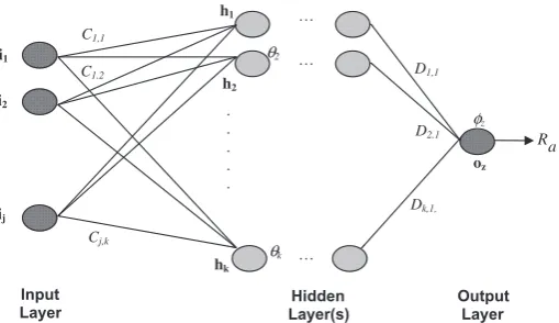
An illustration of the ANN structure used to develop a model forRais given inFig. 3.

FromFig. 3, considering the multilayer feedforward training network with one hidden layer is applied, the net input to

unitkin the hidden layer is expressed in Eq.(7)

net hidden¼X

J

j¼1

Cj;kijþhk; ð7Þ

whereJis number of nodes of the input layer,Cj,kis the weight between the input nodes and hidden nodes,ijis the value of

the input which consists of cutting conditions such as speed, feed rate and rake angle of the experimental sample, andhkis

the biases on the hidden nodes.

Consequently, the net input to unitzin the output layer is expressed in Eq.(8)

net output¼X

K

k¼1

Dk;zhkþ/z; ð8Þ

Fig. 2.Illustration of up and down milling processes.

a R

… … …

i1

i2

ij

oz

φz

Dk,1,

D2,1

D1,1

hk

h2

h1

Cj,k

θ2

θk

C1,2

C1,1

θ

θ θ

θ

o .

.

. . . . .

Hidden Layer(s)

Output Layer Input

Layer

(4)

whereKis number of nodes of the hidden layer,Dk,zis the weight between hidden and output nodes,hkis the value of the

output for hidden nodes, and/zis the biases on the output nodes.

From Eqs.(7) and (8), the output for hidden nodes can be given as Eq.(9), and the output for output nodes can be given as

Eq.(10)

hk¼fðnet hiddenÞ; ð9Þ

oz¼fðnet outputÞ ¼Ra; ð10Þ

wherefis the transfer function to predictRavalue.

3. Experimental data of the case studies

The machining experiment by Mohruni[20]to measure theRavalue in the end milling was considered in this study. The

work piece used in the experiments was an annealed alpha–beta titanium alloy, Ti–6Al–4V (Ti-64). The chemical

composi-tion of the Ti–6Al–4V are listed inTable 1. Three types of end mills were used in the experiments, namely uncoated carbide

(WC-Co) and two TiAlN base coated carbide tools which include common PVD-TiAlN coated carbide tool and PVD with

en-riched Al-content TiAlN coated carbide tools (also called Supernitride coating or SNTR). The composition and properties of

these cutting tools are illustrated inTable 2.

3.1. Experimental design

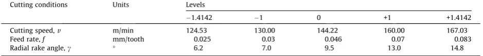
Three cutting conditions are considered for end milling machining process. They are cutting speed, feed rate and radial

rake angle. Experimental design for the end milling process is given inTable 3. From this table, the ﬁve levels of cutting

con-dition of experimental design are1.4142,1, 0, +1 and +1.4142. The whole experiments were carried out under ﬂood

con-ditions (6% concentration of water base coolants) with 5 mm constant axial depth of cut and 2 mm constant radial depth of cut.

Table 1

Chemical composition of Ti–6Al4V.

Al 6.37

V 3.89

Fe 0.16

C 0.002

Mo <0.01

Mn <0.01

Si <0.01

Ti Balance

Table 2

Properties of the cutting tool used in the experiments.

Tool type Uncoated TiAlN coated SNTRcoated

Substrate (wt%) WC 94 94 94

Co 6 6 6

Properties Grade K30 K30 K30

Grain size (lm) 0.5 0.5 0.5

Coating Process – PVD-HIS PVD-HIS

Coating thickness – Monolayer (3–4lm) Multilayer (1–8lm)

Film composition (mol-%AIN) – Approx. 54 Approx. 65–67

Table 3

Levels of cutting condition for end milling.

Cutting conditions Units Levels

1.4142 1 0 +1 +1.4142

Cutting speed,v m/min 124.53 130.00 144.22 160.00 167.03

Feed rate,f mm/tooth 0.025 0.03 0.046 0.07 0.083

(5)

3.2. Experimental results

A total of 24 experimental trials were executed based on eight data of two levels DOE 2k_{full factorial, four center and}

twelve axial points. AllRavalues were collected during actual machining for the three type of cutting tools, uncoated, TiA1N

coated and SNTRcoated cutting tools, are shown inTable 4.

4. Development of regression model

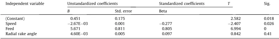
Regression models for each cutting tool are developed using SPSS software based on the experimental data given inTable

4. The coefﬁcients value of modeled independent variable for uncoated, TiA1N coated and SNTRcoated cutting tools are given

inTables 5–7, respectively.

By transferring the coefﬁcients value of independent variable (Tables 5–7) into Eq.(6), the regression model for each

cut-ting tool could be written as follows:

^

y1¼R^a uncoated¼0:4510:00267x1þ5:671x2þ0:0046x3; ð11Þ

^

y2¼^Ra TiA1N¼0:2920:000855x1þ5:383x20:00553x3; ð12Þ

^

y3¼^Ra SNTR¼0:2370:00175x1þ8:693x20:00159x3 ð13Þ

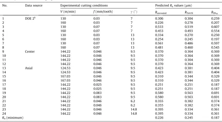
Eqs.(11)–(13)are used to calculate the predictedRavalues, and the results are summarized inTable 8. Then,Ravalues of the

experimental data (Table 4) and the predictedRavalues of regression model (Table 8) are compared. The line pattern data of

Rareal machining vs. predictedRaregression model in shown inFig. 4.

Table 4

ExperimentalRavalues for end milling.

No. Data source Setting values of experimental cutting conditions ExperimentalRavalue (lm)

v(m/min) f(mm/tooth) c(°) Ra_uncoated Ra_TiA1N RaSNTR

1 DOE 2k

130 0.03 7 0.365 0.32 0.284

2 160 0.03 7 0.256 0.266 0.196

3 130 0.07 7 0.498 0.606 0.668

4 160 0.07 7 0.464 0.476 0.624

5 130 0.03 13 0.428 0.260 0.280

6 160 0.03 13 0.252 0.232 0.190

7 130 0.07 13 0.561 0.412 0.612

8 160 0.07 13 0.512 0.392 0.576

9 Center 144.22 0.046 9.5 0.464 0.324 0.329

10 144.22 0.046 9.5 0.444 0.380 0.416

11 144.22 0.046 9.5 0.448 0.460 0.352

12 144.22 0.046 9.5 0.424 0.304 0.400

13 Axial 124.53 0.046 9.5 0.328 0.360 0.344

14 124.53 0.046 9.5 0.324 0.308 0.320

15 167.03 0.046 9.5 0.236 0.340 0.272

16 167.03 0.046 9.5 0.240 0.356 0.288

17 144.22 0.025 9.5 0.252 0.308 0.230

18 144.22 0.025 9.5 0.262 0.328 0.234

19 144.22 0.083 9.5 0.584 0.656 0.640

20 144.22 0.083 9.5 0.656 0.584 0.696

21 144.22 0.046 6.2 0.304 0.300 0.361

22 144.22 0.046 6.2 0.288 0.316 0.360

23 144.22 0.046 14.8 0.316 0.324 0.368

24 144.22 0.046 14.8 0.348 0.396 0.360

Ra(minimum) 0.236 0.232 0.190

Table 5

Coefﬁcients values for uncoated cutting tool.

Independent variable Unstandardized coefﬁcients Standardized coefﬁcients T Sig.

B Std. error Beta

(Constant) 0.451 0.175 2.582 0.018

Speed 2.67E03 0.001 0.277 2.407 0.026

Feed 5.671 0.811 0.805 6.994 0

(6)

As illustrated inFig. 4, the three generated graphs for uncoated, TiA1N coated and SNTRcoated cutting tools gave a similar

pattern forRavalues between the experimental data and regression model data. Therefore, the assumption could be made is

that all cutting tools have given a good prediction in estimating the predictedRavalues.

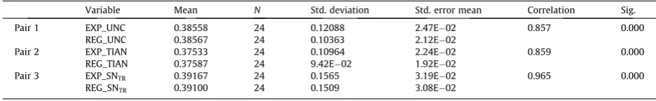
In selecting the best regression model, a convenient approach is to evaluate all possible regression models[21]. In this

study, thettest is conducted to determine the cutting tool that it deals with the best end milling regression model. The

paired-samplettest using SPSS software was conducted to determine the best regression model and the results were

sum-marized inTables 9 and 10.

Table 9 shows that all three pairs of experimental data and regression modeling data are positively correlated,

r(N= 24) = 0.857 for pair 1,r(N= 24) = 0.859 for pair 2, andr(N= 24) = 0.965 for pair 3. FromTable 10, it can be seen that

the mean Ra value for pair 1 increased from the experimental result to the uncoated regression model result by

0.0000833,t(23) =0.007,p= 0.995. The 95% conﬁdence interval ranges from0.0264 to 0.0263 (including zero). Therefore,

the two means of experimental result and regression model results are not signiﬁcantly different from each other. The mean

Table 6

Coefﬁcients values for TiA1N coated cutting tool.

B Std. error Beta

(Constant) 0.292 0.158 1.85 0.079

Speed 8.55E04 0.001 0.098 0.854 0.403

Feed 5.383 0.731 0.843 7.36 0

Radial rake angle 5.53E03 0.005 0.129 1.122 0.275

Table 7

Coefﬁcients values for SNTRcoated cutting tool.

B Std. Error Beta

(Constant) 0.237 0.116 2.042 0.055

Speed 1.75E03 0.001 0.14 2.368 0.028

Feed 8.693 0.539 0.954 16.143 0

Radial rake angle 1.59E03 0.004 0.026 0.437 0.667

Table 8

PredictedRavalues of end milling regression model.

No. Data source Experimental cutting conditions PredictedRavalues (lm)

V(m/min) f(mm/tooth) cð_Þ _^

Runcoated ^RTiA1N ^RSNTR

1 DOE 2k ₁₃₀ _0.03 ₇ _0.306 _0.304 _0.259

2 160 0.03 7 0.226 0.278 0.207

3 130 0.07 7 0.533 0.519 0.607

4 160 0.07 7 0.453 0.493 0.554

5 130 0.03 13 0.334 0.270 0.250

6 160 0.03 13 0.254 0.245 0.197

7 130 0.07 13 0.561 0.486 0.597

8 160 0.07 13 0.481 0.460 0.545

9 Center 144.22 0.046 9.5 0.370 0.364 0.369

10 144.22 0.046 9.5 0.370 0.364 0.369

11 144.22 0.046 9.5 0.370 0.364 0.369

12 144.22 0.046 9.5 0.370 0.364 0.369

13 Axial 124.53 0.046 9.5 0.423 0.381 0.404

14 124.53 0.046 9.5 0.423 0.381 0.404

15 167.03 0.046 9.5 0.310 0.344 0.329

16 167.03 0.046 9.5 0.310 0.344 0.329

17 144.22 0.025 9.5 0.251 0.251 0.187

18 144.22 0.025 9.5 0.251 0.251 0.187

19 144.22 0.083 9.5 0.580 0.563 0.691

20 144.22 0.083 9.5 0.580 0.563 0.691

21 144.22 0.046 6.2 0.355 0.382 0.374

22 144.22 0.046 6.2 0.355 0.382 0.374

23 144.22 0.046 14.8 0.395 0.334 0.361

24 144.22 0.046 14.8 0.395 0.334 0.361

(7)

Ravalue for the pair 2 also increased from the experimental result to the TiA1N coated regression model result by 0.000542,

t(23) =0.047,p= 0.963. The 95% conﬁdence interval ranges from0.0243 to 0.0232 (including zero), which also proves

Uncoted Cutting Tool

0.000 0.100 0.200 0.300 0.400 0.500 0.600 0.700

1 2 3 4 5 6 7 8 9 10 11 12 13 14 15 16 17 18 19 20 21 22 23 24

Ra value

Experimental Data Regression Model

TiA1N Coated Cutting Tool

0.000 0.100 0.200 0.300 0.400 0.500 0.600 0.700

1 2 3 4 5 7 8 9 10 11 12 13 14 15 16 17 18 19 20 21 22 23 24

Samples

Samples Samples

SNTR Coated Cutting Tool

0.000 0.100 0.200 0.300 0.400 0.500 0.600 0.700 0.800

1 2 3 4 5 6 7 8 9 10 11 12 13 14 15 16 17 18 19 20 21 22 23 24

6

Fig. 4.Experimental vs. regression forRavalues.

Table 9

Statistics and correlations (experimental vs. regression).

Variable Mean N Std. deviation Std. error mean Correlation Sig.

Pair 1 EXP_UNC 0.38558 24 0.12088 2.47E02 0.857 0.000

REG_UNC 0.38567 24 0.10363 2.12E02

Pair 2 EXP_TIAN 0.37533 24 0.10964 2.24E02 0.859 0.000

REG_TIAN 0.37587 24 9.42E02 1.92E02

Pair 3 EXP_SNTR 0.39167 24 0.1565 3.19E02 0.965 0.000

(8)

that the two means are not signiﬁcantly different from each other. By looking at the pair 3 inTable 10, it can be seen that the

mean Ra value however reduced from experimental result to the SNTR coated regression model result by 0.000667,

t(23) = 0.079,p= 0.938. The 95% conﬁdence interval ranges from0.0168 to 0.0181 (including zero). Therefore, the two

means too are not signiﬁcantly different from each other.

As a conclusion, based on the results of the paired-samplettest, it could be summarized that the SNTRcoated cutting tool

has given the highest positive correlation and is the only pair that gave a reduced meanRavalue from the experimental

re-sult. Thus, it can be concluded that the predictedRaequation of SNTRcoated cutting tools, Eq.(13), is proposed as

optimi-Table 10

Paired samples test (experimental vs. regression).

Pair Paired differences T Df Sig.

(2-tailed)

Mean Std.

deviation

Std. error mean

95% Conf. inter. of the difference

Lower Upper

Pair 1 EXP_UNC and REG_UNC 8.33E05 6.24E02 1.27E02 2.64E02 2.63E02 0.007 23 0.995 Pair 2 EXP_TIAN and REG_TIAN 5.42E04 5.62E02 1.15E02 2.43E02 2.32E02 0.047 23 0.963 Pair 3 EXP_SNTRand REG_SNTR 6.67E04 4.13E02 8.43E03 1.68E02 1.81E02 0.079 23 0.938

(9)

zation objective function for end milling process. The minimum predicted surface roughness value of SNTRcoated cutting

tool that is selected as the best regression model is 0.187

l

m (the 17th and 18th row ofTable 8). The cutting conditions

val-ues that lead to minimum predicted surface roughness value of SNTRcoated are:v= 144.22 m/min,f= 0.025 mm/tooth and

c

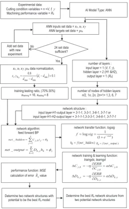
¼9:5_.

5. Development of ANN model

The eight selection inﬂuencing factors in developing the ANN model are given as follows:

(i) The ANN network structure to give the best prediction result. (ii) The ratio of training and testing data for the developed ANN model.

(iii) The normalization of the input/output data made with the available experimental sample size data. (iv) The network algorithm to give the best prediction result.

(v) The transfer function to give the best prediction result.

(vi) The performance functions to give a low error rate in the predicted value.

(vii) The training function to give a low error rate in the response value for the developed ANN model. (viii) The learning function to give a low error rate in the response value for the developed ANN model.

Considering the eight inﬂuencing factors above, the ﬂow of development of the ANN model for end milling is illustrated in

Fig. 5.

Normalized machining cutting condition values are used as the inputs, and normalized machining performance value is

used as the target in the modeling process. A normalization equation suggested by Sanjay and Jyothi[22]as given as follows:

xi¼

0:8

dmaxdminð

didminÞ þ0:1 ð14Þ

Considering the normalization equation in Eq.(11), the normalized values for end milling experimental data are calculated

and given inTable 11. From 24 normalized experimental sets of data, they will be separated into two groups which are

train-ing and testtrain-ing set data. Four sets of center data (the 9th to 12th sets of experimental data) and twelve sets of axial data (the

13th to the last sets of experimental data), giving a total of 16 sets of data, were chosen as the training set data. DOE 2k_data

(the ﬁrst eight experimental data) with a total of eight sets of data will be used as the testing data.

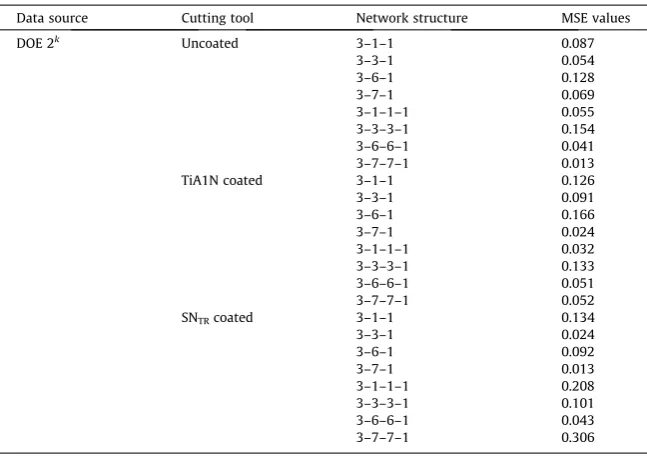
With the ANN Matlab toolbox (learning rate = 0.01, and momentum rate = 0.05), the modeling result (surface roughness

predicted value) for the training set data is summarized inTable 12. The MSE values for the testing set data is given in

Table 11

Normalized values of machining data.

No. Data source xi yRa

xspeed xfeed xrake angle yRauncoated yRaTiA1N yRaSNTR

1 DOE 2k _0.203 _0.169 _0.174 _0.346 _0.266 _0.249

2 0.768 0.169 0.174 0.138 0.164 0.109

3 0.203 0.721 0.174 0.599 0.806 0.856

4 0.768 0.721 0.174 0.534 0.560 0.786

5 0.203 0.169 0.733 0.466 0.153 0.242

6 0.768 0.169 0.733 0.130 0.100 0.100

7 0.203 0.721 0.733 0.719 0.440 0.767

8 0.768 0.721 0.733 0.626 0.402 0.710

9 Center 0.471 0.390 0.407 0.534 0.274 0.320

10 0.471 0.390 0.407 0.496 0.379 0.457

11 0.471 0.390 0.407 0.504 0.530 0.356

12 0.471 0.390 0.407 0.458 0.236 0.432

13 Axial 0.100 0.390 0.407 0.275 0.342 0.343

14 0.100 0.390 0.407 0.268 0.243 0.306

15 0.900 0.390 0.407 0.100 0.304 0.230

16 0.900 0.390 0.407 0.108 0.334 0.255

17 0.471 0.100 0.407 0.130 0.243 0.163

18 0.471 0.100 0.407 0.150 0.281 0.170

19 0.471 0.900 0.407 0.763 0.900 0.811

20 0.471 0.900 0.407 0.900 0.764 0.900

21 0.471 0.390 0.100 0.230 0.228 0.370

22 0.471 0.390 0.100 0.199 0.258 0.369

23 0.471 0.390 0.900 0.252 0.274 0.381

24 0.471 0.390 0.900 0.313 0.409 0.369

(10)

Table 12

Predicted values of ANN training.

No. Data source

Uncoated TiA1N coated SNTRcoated

3–1– 1

3–3– 1

3–6– 1

3–7– 1

3–1– 1–1

3–3– 3–1

3–6– 6–1

3–7– 7–1

3–1– 1

3–3– 1

3–6– 1

3–7– 1

3–1– 1–1

3–3– 3–1

3–6– 6–1

3–7– 7–1

3–1– 1

3–3– 1

3–6– 1

3–7– 1

3–1– 1–1

3–3– 3–1

3–6– 6–1

3–7– 7–1

1 Center 0.069 0.185 0.348 0.291 0.224 0.406 0.417 0.409 0.255 0.334 0.160 0.342 0.229 0.387 0.372 0.296 0.308 0.366 0.519 0.317 0.081 0.387 0.385 0.412 2 0.069 0.185 0.348 0.291 0.224 0.406 0.417 0.409 0.255 0.334 0.160 0.342 0.229 0.387 0.372 0.296 0.308 0.366 0.519 0.317 0.081 0.387 0.385 0.412 3 0.069 0.185 0.348 0.291 0.224 0.406 0.417 0.409 0.255 0.334 0.160 0.342 0.229 0.387 0.372 0.296 0.308 0.366 0.519 0.317 0.081 0.387 0.385 0.412 4 0.069 0.185 0.348 0.291 0.224 0.406 0.417 0.409 0.255 0.334 0.160 0.342 0.229 0.387 0.372 0.296 0.308 0.366 0.519 0.317 0.081 0.387 0.385 0.412 5 Axial 0.033 0.328 0.277 0.225 0.197 0.481 0.346 0.441 0.565 0.576 0.449 0.043 0.474 0.390 0.463 0.157 0.769 0.425 0.057 0.006 0.057 0.457 0.317 0.297 6 0.033 0.328 0.277 0.225 0.197 0.481 0.346 0.441 0.565 0.576 0.449 0.043 0.474 0.390 0.463 0.157 0.769 0.425 0.057 0.006 0.057 0.457 0.317 0.297 7 0.362 0.454 0.295 0.276 0.357 0.241 0.095 0.031 0.118 0.284 0.333 0.609 0.130 0.390 0.247 0.438 0.088 0.302 0.150 0.648 0.267 0.355 0.509 0.412 8 0.362 0.454 0.295 0.276 0.357 0.241 0.095 0.031 0.118 0.284 0.333 0.609 0.130 0.390 0.247 0.438 0.088 0.302 0.150 0.648 0.267 0.355 0.509 0.412 9 0.262 0.240 0.027 0.255 0.189 0.283 0.247 0.456 0.098 0.232 0.157 0.319 0.127 0.457 0.374 0.135 0.104 0.640 0.159 0.254 0.427 0.386 0.330 0.097 10 0.262 0.240 0.027 0.255 0.189 0.283 0.247 0.456 0.098 0.232 0.157 0.319 0.127 0.457 0.374 0.135 0.104 0.640 0.159 0.254 0.427 0.386 0.330 0.097 11 0.028 0.524 0.648 0.653 0.889 0.383 0.615 0.337 0.902 0.469 0.670 0.432 0.762 0.325 0.406 0.801 0.877 0.220 0.461 0.567 0.051 0.333 0.464 0.759 12 0.028 0.524 0.648 0.653 0.889 0.383 0.615 0.337 0.902 0.469 0.670 0.432 0.762 0.325 0.406 0.801 0.877 0.220 0.461 0.567 0.051 0.333 0.464 0.759 13 0.127 0.101 0.578 0.528 0.211 0.404 0.013 0.436 0.227 0.388 0.640 0.138 0.101 0.406 0.540 0.218 0.422 0.294 0.731 0.117 0.238 0.409 0.174 0.231 14 0.127 0.101 0.578 0.528 0.211 0.404 0.013 0.436 0.227 0.388 0.640 0.138 0.101 0.406 0.540 0.218 0.422 0.294 0.731 0.117 0.238 0.409 0.174 0.231 15 0.038 0.624 0.066 0.076 0.262 0.266 0.890 0.059 0.310 0.100 0.277 0.447 0.876 0.305 0.330 0.525 0.183 0.219 0.009 0.834 0.053 0.332 0.468 0.432 16 0.038 0.624 0.066 0.076 0.262 0.266 0.890 0.059 0.310 0.100 0.277 0.447 0.876 0.305 0.330 0.525 0.183 0.219 0.009 0.834 0.053 0.332 0.468 0.432 Minimum

(Ra)

0.028 0.101 0.027 0.076 0.189 0.241 0.013 0.031 0.098 0.100 0.157 0.043 0.101 0.305 0.247 0.135 0.088 0.219 0.009 0.006 0.051 0.332 0.174 0.097

A.M.

Zain

et

al.

/Applied

Mathematical

Modelling

36

(2012)

(11)

Table 13. The MSE plot results of Matlab optimization toolbox, with single hidden layer and two hidden layers of network

structure, for each cutting tool are given inFigs. 6 and 7, respectively.

In order to determine the best ANN model, overall, four factors are given consideration and separated into two parts. The ﬁrst part is determination of the network structure with potential to be the best ANN prediction model. The second part is determination of the best network structure from two potential network structures.

For the ﬁrst factor,Fig. 8shows six graphs which represent the line patterns of the data between the ANN targets and the

ANN outputs for uncoated, TiA1N coated, and SNTRcoated for ANN model with single hidden layer and two hidden layers.

According to the graphs inFig. 8, summary of the similarities in the line pattern criterion is given in the third column of

Table 14. The forth column ofTable 14presents the result of thettest which gives the correlation value between the ANN targets and the ANN outputs which is the second factor to be considered in determining the two networks with the potential to be the best ANN model.

Supported by quite similar of the pattern line and the high positive correlation values, according toTable 14, it could be

stated that the two networks with the potential to be the best ANN model are:

(i) The 3–7–7–1 network structure of TiA1N coated cutting tool.

(ii) The 3–7–7–1 network structure of SNTRcoated cutting tool.

Consequently, these two network structures will be considered with the next two factors to determine which network struc-ture offers the best ANN model. In order to state the network strucstruc-ture that is labeled as the best ANN model, the ﬁrst

con-sideration factor is by referring to the last row ofTable 12, predictedRavalue of ANN training. It was obtained that the

minimum predictedRavalue in the testing phase for the 3–7–7–1 network structure of TiA1N coated and the 3–7–7–1

net-work structure of SNTRcoated are 0.135 and 0.097, respectively.

The second consideration factor is by referring to the last column ofTable 13, MSE values of ANN training. It was obtained

that the MSE value in the testing phase for the 3–7–7–1 network structure of TiA1N coated and the 3–7–7–1 network

struc-ture of SNTRcoated are 0.052 and 0.306, respectively.

With the two consideration factors above, it was found that the 3–7–7–1 network structure of TiA1N coated gave a

smal-ler value in terms of the minimum predictedRa; however the 3–7–7–1 network structure of SNTRcoated gave a smaller value

in terms of the minimum MSE value. Therefore, to decide the best model, this study considers to the higher correlation value

of the network structure. Since the 3–7–7–1 network structure of SNTRcoated has given a higher correlation value, it was

selected to be the best ANN model.

The minimum normalized predictedRavalue of SNTRcoated that selected as the best ANN model is 0.097 (the ﬁfth and

sixth rows: axial data ofTable 12). The normalized cutting condition values that lead to minimum predictedRavalue for SNTR

coated are:

_v

= 0.471,f= 0.100, and

c

= 0.407 (the ﬁfth and sixth rows: axial data ofTable 12). In terms of actual machining

values, the cutting conditions values that lead to the minimumRausing SNTRcoated are

v

= 144.22 m/min,f= 0.025 mm/

tooth, and

c

¼9:5_{(the ﬁfth and sixth rows: axial data of}_{Table 4}_).

Table 13

MSE values of ANN testing.

Data source Cutting tool Network structure MSE values

DOE 2k

Uncoated 3–1–1 0.087

3–3–1 0.054

3–6–1 0.128

3–7–1 0.069

3–1–1–1 0.055

3–3–3–1 0.154

3–6–6–1 0.041

3–7–7–1 0.013

TiA1N coated 3–1–1 0.126

3–3–1 0.091

3–6–1 0.166

3–7–1 0.024

3–1–1–1 0.032

3–3–3–1 0.133

3–6–6–1 0.051

3–7–7–1 0.052

SNTRcoated 3–1–1 0.134

3–3–1 0.024

3–6–1 0.092

3–7–1 0.013

3–1–1–1 0.208

3–3–3–1 0.101

3–6–6–1 0.043

(12)

To estimate the actual value for the minimumRavalues, the normalization equation given in Eq.(11)is modiﬁed.

Calcu-lation for the expected actual value ofRais given as follows:

Uncoated

TiA1N coated

SN

TR

coated

3-1-1 network structure

0 10 20 30 40 50 60 70 80 90 100

10-2 10-1 100 100 Epochs T rai ni ng-B lue

Performance is 0.0871968, Goal is 0

3-1-1 network structure

0 10 20 30 40 50 60 70 80 90 100

10-1 100 100 Epochs T rai ni n g -B lu e

3-1-1 network structure

0 10 20 30 40 50 60 70 80 90 100

10-1 100 100 Epochs Tr a in in g -B lu e

3-3-1 network structure

0 10 20 30 40 50 60 70 80 90 100

10-2 10-1 100 Epochs T ra ini ng-B lu e

3-3-1 network structure

0 10 20 30 40 50 60 70 80 90 100

10-2 10-1 100 100 Epochs T rai ni ng-B lue

3-3-1 network structure

0 10 20 30 40 50 60 70 80 90 100

10-2 10-1 100 Epochs Tr a in in g -B lu e

3-6-1 network structure

0 10 20 30 40 50 60 70 80 90 100

3-6-1 network structure

0 10 20 30 40 50 60 70 80 90 100

3-6-1 network structure

0 10 20 30 40 50 60 70 80 90 100

10-2 10-1 100 100 Epochs T rai ni n g -B lu e

3-7-1 network structure

0 10 20 30 40 50 60 70 80 90 100

10-2 10-1 100 Epochs T rai ni ng-B lue

3-7-1 network structure

0 10 20 30 40 50 60 70 80 90 100

10-2 10-1 100 Epochs Tr a in in g -B lu e

3-7-1 network structure

0 10 20 30 40 50 60 70 80 90 100

10-2 10-1 100 Epochs T rai ni n g -B lu e

(13)

di¼

ðyRa0:1ÞðdmaxdminÞ

0:8 þdmin¼

ð0:0970:1Þð0:6960:190Þ

0:8 þ0:190¼0:1881030:188

l

m ð15Þ

Uncoated

TiA1N coated

SN

TR

coated

3-1-1-1 network structure

0 10 20 30 40 50 60 70 80 90 100 10-2 10-1 100 Epochs Tr a in in g -B lu e

3-1-1-1 network structure

0 10 20 30 40 50 60 70 80 90 100 10-1 100 100 Epochs T raining-B lue

3-3-3-1 network structure

0 10 20 30 40 50 60 70 80 90 100 10-1 100 100 Epochs Tr a in in g -B lu e

3-3-3-1 network structure

0 10 20 30 40 50 60 70 80 90 100 10-1 100 100 Epochs T rai ni ng-B lu e

3-3-3-1 network structure

0 10 20 30 40 50 60 70 80 90 100 10-1 100 100 Epochs T rai ni ng-B lu e

3-6-6-1 network structure

0 10 20 30 40 50 60 70 80 90 100 10-2 10-1 100 Epochs T ra ini ng-B lu e

3-7-7-1 network structure

0 10 20 30 40 50 60 70 80 90 100 10-2 10-1 100 Epochs T rai ni n g -B lu e

3-7-7-1 network structure

0 10 20 30 40 50 60 70 80 90 100 10-1 100 100 Epochs Tr a in in g -B lu e

(14)

Predicted value of single hidden layer ANN for uncoated cutting tool

0 0.2 0.4 0.6 0.8 1

1 2 3 4 5 6 7 8 9 10 11 12 13 14 15 16

ANN target ANN predicted 3-1-1 ANN predicted 3-3-1

ANN predicted 3-6-1 ANN predicted 3-7-1

Predicted value of single hidden layer ANN for TiAIN coated cutting tool

0 0.2 0.4 0.6 0.8 1

1 2 3 4 5 6 7 8 9 10 11 12 13 14 15 16

Predicted values of single hidden layer ANN for SNTR coated cutting tool

0 0.2 0.4 0.6 0.8 1

1 2 3 4 5 6 7 8 9 10 11 12 13 14 15 16

Predicted value of two hidden layers ANN for uncoated cutting tool

0 0.2 0.4 0.6 0.8 1

1 2 3 4 5 6 7 8 9 10 11 12 13 14 15 16

ANN target ANN predicted 3-1-1-1 ANN predicted 3-3-3-1

ANN predicted 3-6-6-1 ANN predicted 3-7-7-1

Predicted value of two hidden layers ANN for TiAIN coated cutting tool

0 0.2 0.4 0.6 0.8 1

1 2 3 4 5 6 7 8 9 1011 1213 14 15 16

Predicted value of two hidden layers ANN for SNTR coated cutting tool

0 0.2 0.4 0.6 0.8 1

1 2 3 4 5 6 7 8 9 10 11 12 13 14 15 16

Fig. 8.ANN target vs. ANN output.

Table 14

Correlation values and similarity of the line pattern of ANN model.

Cutting tool Pair of variables Pattern line Correlation value

Uncoated Experimental-ANN 311 Less similar .652

Experimental-ANN 331 Less similar .158

Experimental-ANN 3–1–1–1 Quite similar .724

Experimental-ANN 3–3–3–1 Less similar .422

TiA1N coated Experimental-ANN 311 Quite similar .780

SNTRcoated Experimental-ANN 311 Quite similar .728

Table 15

Statistics and correlations (experimental data vs. ANN training of 3–7–7–1 structure).

Variable Mean N Std. deviation Std. error mean Correlation Sig.

EXP_SNTR 0.38950 16 0.20067 5.0168E02 0.869 0.000

(15)

6. Validation and evaluation of results

It was observed inTable 8, the minimum predictedRavalue of the best regression model is 0.187

l

m, given by SNTR

coated cutting tool. The process of validation for the regression model, basically, could refer to the paired-samplettest

con-ducted in Section4in determining the best end milling model. According to the last row ofTables 9 and 10, it was proven

that the mean Ra value reduced from experimental result to the SNTR coated regression model result by 0.000667,

t(23) = 0.079,p= 0.938. The 95% conﬁdence interval ranges from0.0168 to 0.0181 (including zero). Therefore, the two

means, experimental and SNTRcoated regression model are not signiﬁcantly different from each other.

The results of the paired-samplettest for SNTRexperimental data coupled with predicted value of the ANN 3–7–7–1 SNTR

coated (the best ANN model) training data are summarized inTables 15 and 16as follows.

According toTables 15 and 16, it was proven that the meanRavalue reduced from SNTRcoated experimental result to the

SNTRcoated ANN model result by 0.008,t(15) = 0.320, p= 0.869. The 95% conﬁdence interval ranges from0.04531 to

0.061317 (including zero). Therefore, the two means, SNTRcoated experimental and SNTRcoated ANN 3–7–7–1 model are

not signiﬁcantly different from each other. In other words, the average surface roughness predicted value of the ANN 3–

7–7–1 SNTRcoated (the best ANN model) is similar to the average actual surface roughness found through experiment.

Consequently, focused on the predictedRavalue, the evaluation of the developed regression and ANN models are given as

follows:

(a) Experimental data vs. regression.

As shown inTable 4, the minimumRavalue among all the cutting tools for experimental data is 0.190

l

m, given by

SNTRcutting tool. Therefore, withRa= 0.187

l

m (Table 8), it can be stated that the regression model has given a lower

minimum value of theRacompared to experimental data by about 0.003

l

m.

(b) Experimental data vs. ANN.

WithRa= 0.188

l

m for ANN (Eq.(12)) andRa= 0.190

l

m for experimental data, it can be stated that ANN has given a

lower minimum value of the predictedRaby about 0.002

l

m.

(c) Regression vs. ANN.

WithRa= 0.187

l

m for regression, it can be stated that regression has given a lower minimum value of theRa

com-pared to ANN by about 0.001

l

m.

7. Conclusion

This study has applied two techniques for estimating the minimum machining performance value. First technique,

devel-opment of regression model, has been discussed in Section4. Second technique, development of ANN model, has been

dis-cussed in Section5.

According to the evaluation of the results discussed in Section6,Table 17summarizes results of the minimum machining

performance values of experimental data, regression, and ANN. Consequently,Table 18indicates the reduction percentage of

the surface roughness that was given by the regression and ANN models when compared to the results of experimental data.

According toTable 17, it is clear that this study has found that both modeling approaches have outperformed the

min-imumRavalue of the experimental. FromTable 18, it was found that both models have reduced the minimumRavalue of

experimental data at about 1.57% and 1.05% respectively. Overall, it could be stated that the regression has given a better

result when compared to ANN in predicting the minimumRavalue.

Table 16

Paired samples test (experimental data vs. ANN training of 3–7–7–1 structure).

Pair Paired differences T Df Sig. (2-tailed)

Mean Std. deviation Std. error mean 95% Conf. inter. of the difference

Lower Upper

EXP_SNTRand ANN_ SNTR 8.0000E03 0.10006 2.5015E02 4.5317E02 6.1317E02 0.320 15 0.754

Table 17

Minimum value of surface roughness.

Approach MinimumRa(lm)

Experimental 0.190

Regression 0.187

ANN 0.188

GA[23] 0.1385

(16)

Acknowledgments

Special appreciative to reviewer(s) for useful advices and comments. The authors greatly acknowledge the Research Man-agement Centre, UTM and Ministry of Higher Education (MOHE) for ﬁnancial support through the Exploratory Research Grant Vot. No. 4L003.

References

[1] J.T. Lin, D. Bhattacharyya, V. Kecman, Multiple regression and neural networks analyses in composites machining, Compos. Sci. Technol. 63 (2003) 539– 548.

[2] N. Tosun, L. Ozler, A study of tool life in hot machining using artiﬁcial neural networks and regression analysis method, J. Mater. Process. Technol. 124 (2002) 99–104.

[3] K. Kanlayasiri, S. Boonmung, Effects of wire-EDM machining variables on surface roughness of newly developed DC 53 die steel: design of experiments and regression model, J. Mater. Process. Technol. 192–193 (2007) 459–464.

[4] U. Caydas, A. Hascalik, A study on surface roughness in abrasive waterjet machining process using artiﬁcial neural networks and regression analysis method, J. Mater. Process. Technol. 202 (2008) 574–582.

[5] I. Mukherjee, P.K. Ray, A review of optimization techniques in metal cutting processes, Comput. Ind. Eng. 50 (2006) 15–34.

[6] T. Ozel, Y. Karpat, Predictive modeling of surface roughness and tool wear in hard turning using regression and neural networks, Int. J. Mach. Tools Manuf. 45 (2005) 467–479.

[7] K.M. Rao, G. Rangajanardhaa, R.D. Hanumantha, R.M. Sreenivasa, Development of hybrid model and optimization of surface roughness in electric discharge machining using artiﬁcial neural networks and genetic algorithm, J. Mater. Process. Technol. 209 (2009) 1512–1520.

[8] H.C. Chen, J.C. Lin, Y.K. Yang, C.H. Tsai, Optimization of wire electrical discharge machining for pure tungsten using a neural network integrated simulated annealing approach, Expert Systems Appl. 37 (2010) 7147–7153.

[9] M. Nalbant, H. Gökkaya, I. Toktasß, G. Sur, The experimental investigation of the effects of uncoated, PVD- and CVD-coated cemented carbide inserts and cutting parameters on surface roughness in CNC turning and its prediction using artiﬁcial neural networks, Robot. Comput.-Int. Manuf. 25 (2009) 211– 223.

[10] D. Karayel, Prediction and control of surface roughness in CNC lathe using artiﬁcial neural network, J. Mater. Process. Technol. 209 (2009) 3125–3137. [11] N. Muthukrishnan, J.P. Davim, Optimization of machining parameters of Al/SiC-MMC with ANOVA and ANN analysis, J. Mater. Process. Technol. 209

(2009) 225–232.

[12] D. Venkatesan, K. Kannan, R. Saravanan, A genetic algorithm-based artiﬁcial neural network model for the optimization of machining processes, Neural Comput. Appl. 18 (2009) 135–140.

[13] H. Oktem, An integrated study of surface roughness for modelling and optimization of cutting parameters during end milling operation, Int. J. Adv. Manuf. Technol. 43 (2009) 852–861.

[14] M. Correa, C. Bileza, J. Pamies-Teixeira, Comparison of Bayesian networks and artiﬁcial neural networks for quality detection in machining process, Expert Systems Appl. 36 (2009) 7270–7279.

[15] E.S. Topal, The role of stepover ratio in prediction of surface roughness in ﬂat end milling, Int. J. Mech. Sci. 51 (2009) 782–789.

[16] S. Aykut, M. Demetgul, I.N. Tansel, Selection of optimum cutting condition of cobalt-based superalloy with GONNS, Int. J. Adv. Manuf. Technol. 46 (2010) 957–967.

[17] P. Muñoz-Escalona, P.G. Maropoulos, Artiﬁcial neural network for surface roughness prediction when face milling Al 7075-T7351, J. Mater. Eng. Perform. 19 (2010) 185–193.

[18] A.M. Zain, H. Haron, S. Sharif, Prediction of surface roughness in the end milling machining using artiﬁcial neural network, Expert Systems Appl. 37 (2010) 1755–1768.

[19] Y.H. Tsai, J.C. Chen, S.J. Luu, An in-process surface recognition system based on neural networks in end milling cutting operations, Int. J. Mach. Tools Manuf. 39 (1999) 583–605.

[20] A.S. Mohruni, Performance Evaluation of Uncoated and Coated Carbide Tools When End Milling of Titanium Alloy Using Response Surface Methodology, Thesis Doctor of Philosophy, Universiti Teknologi Malaysia, Skudai, Johor, Malaysia, 2008.

[21] S.H. Yeo, M. Rahman, Y.S. Wong, Towards enhancement of machinability data by multiple regression, J. Mech. Work. Technol. 19 (1989) 85–99. [22] C. Sanjay, C. Jyothi, A study of surface roughness in drilling using mathematical analysis and neural networks. Int. J. Adv. Manuf. Technol. 29 (2006)

846–852.

[23] A.M. Zain, H. Haron, S. Sharif, Application of GA to optimize cutting conditions for minimizing surface roughness in end milling machining process, Expert Systems Appl. 37 (2010) 4650–4659.

[24] A.M. Zain, H. Haron, S. Sharif, Simulated annealing to estimate the optimal cutting conditions for minimizing surface roughness in end milling Ti–6Al– 4V, Mach. Sci. Technol. 14 (2010) 43–62.

Table 18

Reduction percentage of minimum surface roughness.

Approach Reduction ofRa(%)

Modeling Experimental vs. regression 1.57 Experimental vs. ANN 1.05 Optimization Experimental vs. GA 27