A practical implementation of maximum likelihood voting

A Practical Implementation of

Maximum Likelihood Voting

Kalhee Kim, Mladen A. Vouk, and David F. McAllister Department of Computer Science

North Carolina State University Raleigh, NC 27695-8206

Abstract

The Maximum Likelihood Voting (MLV) strategy was recently proposed as one of the most reliable voting methods. The strategy determines the most likely correct result based on the reliability history of each software version. In this paper we first discuss the issues that arise in practical implementation of MLV, such as the question of unrealized outputs, the handling of voting ties, and the issue of inter-version failure correlation. We then present an extended MLV algorithm that

a) uses a dynamic voting strategy which automatically adapts to the number of realized output space categories, and

b) uses component reliability estimates to break voting ties.

We also present an empirical evaluation of the implemented MLV strategy, and we compare it with Recovery Block (RB), N-Version Programming (NVP) and Consensus Recovery Block (CRB) approaches. Our results show that, even under high inter-version failure correlation conditions, our implementation of MLV performs well. In fact, statistically it outperformed all variants of NVP, CRB and RB fault-tolerance strategies that we examined in this study. To the best of our knowledge, this is the first empirical study of the MLV strategy.

Key Words: Maximum Likelihood Voting, N-Version Programming, Consensus Recovery

Block, Consensus Voting, System Reliability, Software Fault-Tolerance, Correlated Failures

* _{Research supported in part by following grants: NASA NAG-1-983 andNGT-70402, MCNC/EPA C94-7050-027}

1. Introduction

The Maximum Likelihood Voting (MLV) strategy was recently proposed [8] as one of the most reliable voting methods for N independently developed functionally equivalent software versions. Unlike classical voting methodologies, such as Majority Voting or Consensus Voting, this technique uses the knowledge of the previous history of each version (its failure probability) to select the correct answer. Assuming that output space is finite and that the version failures are statistically independent, MLV uses the likelihood value of each version output to choose an answer as a correct answer.

Theoretical results [8] show that MLV performs better than classical Majority Voting [2] and Consensus Voting [9]. However, one of the principal concerns with all redundancy based software fault-tolerance strategies is their performance in the presence of correlated failures. Experiments have shown that inter-version failure dependence among independently developed functionally equivalent versions may not be negligible in the context of current software development and testing strategies [11, 7, 5].

By inter-version correlation we mean the following. When two or more functionally equivalent software versions fail on the same input we say that a coincident failure has occurred. If the measured probability of the coincident failures is significantly different from what would be expected by chance,

assuming the failure independence model, then we say that the observed version failures are correlated or dependent [see Appendix I, also 17, 18, 19, 20].

Leung developed the Maximum Likelihood Voting technique assuming failure independence, and he evaluated it using a combination of analytical and simulation approaches [8]. This, and our earlier work with MLV [15], has prompted us to a) explore the MLV implementation issues in detail, and b) extensively investigate its performance under the conditions where inter-version failures are highly correlated. We empirically compared our implementation of MLV with the classical N-version Programming that uses Majority Voting, N-version Programming that uses Consensus Voting, Recovery Block [10, 5] and Consensus Recovery Block [12] techniques (for a brief description of these voting techniques, see Appendix II). We report on the performance of MLV in an environment where inter-version correlation effects can be easily observed, i.e., under the conditions of strong inter-version failure coupling using medium-to-high reliability software versions of the same avionics application as was employed in the Eckhardt et al. [5]

2. Implementation of Maximum Likelihood Voting

2.1. Notation and Assumptions

We use the following notation:

N : number of functionally equivalent software versions. r : output space cardinality.

pi : probability that version i succeeds (is correct), i = 1 ... N. V_i : random variable that represents the output of the version i.

v_i : output value that the random variable V_i takes given an input to version i. (one of r possible program outputs)

Pr{...} : probability of an event.

The following assumptions were used by Leung [8] to define MLV and evaluate it using simulation:

(1) Failures of functionally equivalent versions are statistically independent. (2) The cardinality of the program output space is finite and equal to r.

(3) There are no multiple correct outputs. If a version is successful, of the r possible program outputs, only one is correct.

(4) When a version failure occurs, the incorrect output is one of any r-1 incorrect outputs. All incorrect outputs have the same probability of occurring, i.e., (1-pi)/(r-1).

2.2. The Original Strategy

In his paper, Leung defines Maximum Likelihood Voting strategy in the following way [8]. Let program version i have a unique success state, and let there be r−1 failure states. Let the probability of occurrence of a failure state for program i be 1−pi

r−1, and let ξj be the event where output j is correct. In general, there are r mutually exclusive ξj events (j = 1 ... r). Then, the unconditional joint probability that a particular set of N outputs is produced by the versions can be decomposed into the sum of probabilities that events ξj (j = 1 ... r) occur for the given output set, i.e.:

Pr{V1 =v1,V2 =v2,⋅⋅⋅,VN =vN}= Pr{V1=v1,V2 =v2,⋅⋅⋅,VN =vN,Voracle = j} j=1

r

∑

=

[

]

r

∑ (1)

Pr {_{j i i}}

i

i

V v

p j

p

r j

= =

= −

− ≠

    

if v

if v

i

i

1 1

(2)

Equation (2) specifies probabilities for 2 possible events. One is the probability that the correct answer is j (one particular of the r possible outputs) and version i's output is j. The other is the probability that the correct answer is j and version i's output is one of r−1 possible incorrect outputs.

This allows calculation of the conditional probability that output j is the correct answer, given that a particular set of outputs was obtained:

Pr{Voracle = j|V1=v1,V2=v2,⋅⋅⋅,VN =vN}=

Pr{V₁=v₁,V₂ =v₂,⋅⋅⋅,VN =vN,Voracle = j} Pr{V₁=v₁,V₂ =v₂,⋅⋅⋅,VN =vN}

= = × = × ⋅⋅⋅ × =

= × = × ⋅⋅⋅ × =

[

]

=

∑

Pr { } Pr { } Pr { }

Pr { } Pr { } Pr { }

j j j N N

j j j N N

j r

V v V v V v

V v V v V v

1 1 2 2

1 1 2 2

1

(3)

Once these values are available, the voting routine can choose the output that has the largest probability (likelihood) of being correct based on the received output set. If there is a tie among the largest likelihood values, the voter randomly chooses one among the tied outputs [8]. Leung has also proposed two voting variants, one related to safety issues and the other to timed voting. In this paper, we do not consider these variants.

2.3. Implementation Issues

One of the difficulties in implementing the original MLV algorithm [8] is that it requires calculation of likelihood values for all r possible outputs. However, in many situations computing all r likelihood values may be infeasible because we may not know what r is (except that it is finite and possibly large). Since we need r to estimate the conditional likelihoods defined by equation (3), we have several problems. One is how to assign an r value in the first place, another is how to handle the fact that in many situations only some of the r outputs will be available for decision making, e.g., when N< r.

2.3.1. How to assign output space

number of versions we have developed (i.e., 20 in this case). We call this model MLV-20. The other approach is to make r equal to the effective voter output space observed for each voting run. We call this MLV-dynamic. For example, if we have a 5-version tuple (N=5), and on a particular run we receive back 3 distinct values (2+2+1), then we use r=3 to calculate the likelihoods. We could have made r equal to the number of versions in a tuple, or to some other number. However, we did not notice a significant difference in the performance of the MLV-dynamic and MLV-20 voters.

2.3.2. How to handle unrealized outputs

When voting is based only on the realized values the number of distinct outputs available to the voter for a single test case is not more than N, and in practice it is likely to be less than that. Our earlier work [14] has shown that, in the case of our versions, the effective decision space or effective voter output space (number of distinct outputs submitted to a voter) was usually much less than the number of participating versions (N). Since we voted on floating-point outputs, for which r is very large, effective decision space was also much less than r. Obviously, if a value is returned, it can only come from the realized values. This means that we could limit our calculations only to the realized values (or effective voter output space [14]).

For example, let the system have three versions, and assume that the output space is r =10 for any input. Let a version output vector be [v1=100, v2=102, v3=150]. If we want to calculate the likelihood values for the seven (7) unrealized outputs, what should we do? According to equation (3), any unrealized output space value will have the same numerator in the conditional likelihood equation, i.e., [(1-p1)(1-p2)(1-p3)]/(r-1)3. If all pi are greater than 1/2, the likelihood values for unrealized values will be less than the likelihood values for the realized values, and could be ignored.

The MLV implementation we discuss in this paper is based on the model where only the realized values participate in the decision making. To assess when this could pose a problem, we now examine the conditions under which the MLV (as originally defined) would select an unrealized output.

2.3.3 Condition that an unrealized output is selected as the correct answer

Suppose that we have a system of N functionally equivalent software versions. After outputs from all versions are produced, MLV computes likelihood values for all realized outputs. Then from (3) it follows that the largest likelihood value (Φ is a set containing versions whose member's outputs are all identical) is:

L

=

p

•

1

−

p

r

−

1

i∉Φ∏ i∈Φ∏

P V

{

,

V

⋅⋅⋅

,

V

}

The likelihood value for all unrealized values is:

L

=

1

−

p

r

−

1

i=1 N

∏

P V

{

,

V

⋅⋅⋅

,

V

}

We need to find out the condition where the likelihood value for unrealized values are greater than the maximum likelihood values for realized outputs, i.e.

L

≤

L

⇒

pi•

1− pi

r−1

i∏∉Φ

i∏∈Φ

P V

{

}

≤

1− pi

r−1

i=1

N ∏

P V

{

}

⇒ _p

i•

1−p_i r−1 i∏∉Φ

i∏∈Φ

≤

N

∏

⇒

p_i i∏∈Φ

1−p_i i∏∈Φ

≤

(r−1)Φ

⇒ pi

1− p_i

i∏∈Φ

≤

Hence, as long as pi is greater than 1−pi and r is greater than 2, the maximum (largest) likelihood value among the realized outputs is always greater than the likelihood value for unrealized outputs. In normal MLV operation condition, we expect that pi is greater than 1−pi and r is greater than 2.

The conditions satisfying Lmax ≤Lunrealized can be further specified as the relation among pi, 1−pi and r . The above equation becomes as follows.

⇒ _(r−1)Φ

≤

⇒ −

≤

∈

∏

p

i i i

1 Φ 1

Φ

⇒ −

≤

∈

∏

p

i i i

1 1

Φ Φ

(7) When we assume that the success probabilities (reliabilities) for all version are identical we have:

⇒ −  −



 

 

≤

ln (r ) 1 ln p p

1 1

Φ

Φ

⇒ −  −



 

 

≤

ln (r ) ln p p

1 1

⇒ _r−1

≤

p

⇒(r−1)p ≤ 1−p

⇒p ≤ 1

r (8)

2.3.4. Tie breaking

Another important implementation issue is how to break ties among likelihood values. Leung suggests that such a tie should be broken by random choice [8]. However, random tie breaking may not select the correct output. High inter-version correlation, and use of tolerance-based comparisons, offers many opportunities for inconsistencies and ties. For example, suppose that we have 5 versions and that the outputs from these versions are 3.4, 3.3, 3.3, 3.3, and 3.3. These outputs are identical (within tolerance) if the tolerance is greater than 0.1. Therefore, all compute identical likelihood values. However, if the correct output is 3.5 ±0.1, only the first version has returned an acceptable answer (3.4). Which output among the outputs with identical likelihood values to choose, and how to resolve the issue? Do we return the average value rounded to tolerance, or a weighted average where weighting is the version reliability, or something else? Random tie breaking has one chance in 5 of returning the correct answer. We suggest that another approach may be to choose the answer that was returned by the version that has the highest independently estimated reliability. In our implementations we tried both approaches: random tie breaking, and reliability-based decisions. We have found that, most of the time, reliability-based decisions tend to work better than random tie-breaking. However, we have observed several cases where random decisions gave the correct answer when the most reliable version provided an incorrect response.

The MLV algorithm implementing the tie-breaking strategy based on the reliability history of the versions is given in Appendix III.

2.3.5 Conditions that MLV is identical to NVP-MV and NVP-CV

There are some other issues one has to consider when implementing MLV. For example, is the added complexity of MLV cost-effective? Specifically, when might MLV perform only as well as the classical NVP, and hence it may not be worth implementing? We examine this issue by first considering simple, but practically unrealistic conditions of no-interversion failure correlation and identical version reliability, and then by examining more realistic situations.

pi(1− p)N i− > pj(1−p)N−j i> j

if (assuming that

i >= N+1

2    )

⇒ p

1− p  

 _

i−j

>1

⇒ p> −1 p since i> j

⇒

p

>

1

2

Hence, in binary output space, as long as the versions have identical reliability and p >0.5, MLV is equivalent to NVP-MV. Since Consensus Voting (NVP-CV) reduces to Majority Voting (NVP-MV) in binary output space, MLV is also identical to NVP-CV under the above conditions.

Now consider the situation where r > 2. In this case, NVP-CV performs better than NVP-MV as long as p > 1/r [9, 14]. The relationship between p and r which makes the output with the largest cardinality always have the highest likelihood value is obtained by satisfying the following inequality:

p p r

p p

r i j

i N i

N i

j N j

N j ( ) ( ) ( ) ( ) 1 1 1 1 − − > − − > − − −

− if

⇒ _(r−1)i−j

>(1−p) i−j

pi−j

⇒ _(r−1)i−j p i−j

(1−p)i−j >1

⇒ _(r−1)• p

1−p       i−j

>1

⇒ − •

− >

(r ) p since i > j p

1

1 1

⇒ _r−1>1−p

p

⇒ _r> 1

⇒

_p>1

r (10)

So, when r > 2, MLV will behave exactly like NVP-CV if the reliability of all versions is identical

and it is greater than 1/r.

Of course, in practice it is unlikely that diverse functionally equivalent versions will be perfectly balanced, i.e., will have identical reliability. Unless the testing is exhaustive, or the versions are proved correct, their reliability will be same only to within some statistical tolerance. This means that neither (9) nor (10) will hold, and MLV will have an edge over the "classical" NVP. Furthermore, it is quite likely that at least some of the inter-version failures will be correlated.

In Section 3, using a combination of empirical results and simulations, we discuss the situation where the versions do not have the same reliability and there is inter-version failure correlation.

3. Empirical Performance of MLV

Previous work reported theoretical [e.g., 1, 3, 4, 8, 9, 16, 17] and experimental [e.g., 5, 7, 11, 14,15, 18, 19] results on how the number of versions, version reliability, and inter-version correlation affect system reliability performance of various software fault-tolerance strategies. Economical justifications for software systems with large number of versions has also been discussed in a number of places [e.g., 18, 19], but it is out of the scope of this paper.

In this section we discuss the empirical reliability performance of our implementation of the Maximum Likelihood Voting (MLV-RL-DN1_{) in comparison with N-Version Programming with} Consensus Voting (NVP-CV), N-Version Programming with Majority Voting (NVP-MV), Consensus Recovery Block with either Majority Voting (CRB-MV) or Consensus Voting (CRB-CV), and Recovery Block (RB).

3.1. The Experimental Approach and Metrics

Experimental results are based on a pool of twenty independently developed functionally equivalent programs obtained in a large-scale multiversion software experiment described in several papers [6, 13, 5]. Version sizes range between 2000 and 5000 lines of high level language code. We used the program versions in the state they were immediately after the unit development phase [6], but before they underwent an independent validation (or acceptance) phase of the experiment [5]. This was done to keep the failure probability of individual versions relatively high (and failures

easier to observe), and to retain a considerable number of faults that exhibit mutual failure correlation in order to high-light correlation based effects.

The nature of the faults found in the versions is discussed in detail in two papers [5, 13]. In real situations versions would be rigorously validated before operation, so we would expect that any undesirable events that we observed in our experiments would be less frequent and less pronounced. However, we believe that the mutual performance ordering of different strategies, derived in this study relative to correlation issues, still holds under low correlation conditions. For this study we generated subsets of program N-tuples with: 1) similar average2 _{N-tuple reliability,} and 2) a range of average N-tuple reliabilities. We use the average N-tuple reliability to focus on the behavior of a particular N-tuple instead of the population (pool) from which it was drawn, and to indicate approximate reliability of corresponding mutually independent versions. The subset selection process is described in Appendix IV.

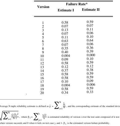
Table 1. Version failure rates

.

Version Failure Rate*

Estimate I Estimate II

1 2 3 4 5 6 7 8 9 10 11 12 13 14 15 16 17 18 19 20 0.58 0.07 0.13 0.07 0.11 0.63 0.07 0.35 0.40 0.004 0.09 0.58 0.12 0.37 0.58 0.58 0.10 0.004 0.58 0.34 0.59 0.07 0.11 0.06 0.10 0.64 0.06 0.36 0.39 0.000 0.10 0.59 0.12 0.38 0.59 0.59 0.09 0.006 0.59 0.33

2 Average N-tuple reliability estimate is defined as –p =

∑

pi

N , and the corresponding estimate of the standard deviation of the sample as ^s =

∑

(–p-^_pi)2

N-1 , where ^p i =

∑

si(j)

In conducting our experiments we considered a number of input profiles and different combinations of versions and output variables. Failure rate estimates based on the three most critical output variables (out of 63 monitored) are shown in Table 1. Two test suites, each containing 500 uniform random input test cases, were used in all estimates discussed in this paper. One suite, which we call Estimate-I, was used to estimate individual version failure rates (probabilities). The other test suite, Estimate-II, was used to investigate the actual behavior of N-tuple systems based on different voting and fault-tolerance strategies.

3.1.1. Smoothing

Because of a) the variance in the average reliability of the N-tuples, b) the sample size (500 test cases), and c) the presence of very highly correlated failures, our experimental system reliability traces tend to be quite uneven and ragged (e.g., Figures 1-3, 5, 6). Since we are primarily interested in the general trends inferred from the theoretical results, we use smoothing to extract these trends from the experimental plots. When smoothing is done with symmetrical K point moving average, the first (K-1)/2 data points and last (K-1)/2 data points from original 50 data points are dropped because there is no symmetrical K points forthose data points.

3.1.2. Diversity

We use the standard deviations of N-tuple reliabilities as a version diversity indicator. For example, a 3 version fault-tolerant system whose individual version reliabilities are (0.91, 0.89, 0.90) is more diverse than the fault-tolerant system whose individual version reliabilities are (0.90, 0.90, 0.90). Throughout this paper, standard deviations of N-tuple reliability should be interpreted as a diversity metric for a particular version combination. Note that the limited size (20) of the population (pool) prohibited us from always obtaining the combinations with standard deviations of N-tuple reliability in the same range for different N's (N=3,5,7).

3.1.3. Acceptance Test

3.1.4. What is the correct answer?

The fault-tolerant software algorithms of interest were invoked for each test case (Estimate II). The outcome was compared with the correct answer obtained from a " golden " program [5, 13] and the frequency of successes and failures for each strategy was recorded.

3.2. MLV vs. Consensus Voting and Majority Voting.

In binary output space Maximum Likelihood Voting and Majority Voting should behave identically when the failure probabilities of all versions are equal and are greater than 1/2. Note that Consensus Voting reduces to Majority Voting in binary output space. For r > 2, MLV is also identical to Consensus Voting if the failure probabilities of all versions are equal and are greater than 1/r. But when r > 2 and the version failure probabilities are not all identical, MLV is expected to offer reliability higher than either Consensus Voting or Majority Voting [8]. In practice, inter-version failure correlation may change this.

3.2.1. How system reliability varies with the number of versions

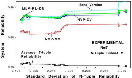
Figure 1 shows smoothed MLV, NVP-CV and NVP-MV reliability trends, and the corresponding average N-tuple reliability vs. N-tuple diversity (i.e., standard deviation of N-tuple reliabilities). This N-tuple subset consists of medium reliability 3-tuples (average reliability between 0.70 and 0.79) of relatively large N-tuple reliability variance. Figures 2 and 3 show the results for 5- and 7-version systems (average reliability also between 0.70 and 0.79). Note that the relative diversity of the three sets is similar (standard deviation of the N-tuple over the average N-tuple reliability).

As the number of versions increases from 3 to 5 to 7, the differences in the performance of MLV, NVP-CV and NVP-MV become less pronounced. This is in agreement with the observations that Leung made based on his simulation work [8]. An illustration of the theoretical behavior is shown in Figure 4. This figure shows simulated3 _{system reliability as the function of the number of versions} under different voting strategies. We used an average N-tuple reliability range of 0.70 to 0.79, and we assumed no inter-version correlation. As in the empirical graphs, we see that for N=5 and beyond the performance gap between MLV and NVP-CV diminishes rapidly, but the one between MLV and NVP-MV remains quite large.

3.2.2. How system reliability varies with the version reliability

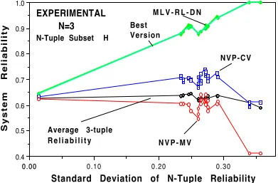
Figure 5 shows the observed reliability of a subset of 3-version systems for a range of average N-tuple reliabilities from 0.55 to 0.64, while Figure 6 shows the behavior for a reliability set in the range 0.85 to 0.94. If we examine Figures 5, 1 and 6, in that order, we get an illustration of what the impact of the average N-tuple reliability is on the system reliability. We can see that in practice MLV reliability is usually at least as good as that of the "best" version, and sometimes it exceeds that of the "best" version (e.g., see Figure 6). On the other hand, NVP-MV and CV usually do not do as well as the "best" version, especially for small N. Note that the "best" version is the particular N-tuple version which exhibits the smallest number of failures among N versions during the actual evaluation run with the suite Estimate-II.

0 . 3 2 1 0 . 3 1 1

0 . 3 0 1 0 . 3 0 1 0.74 0.84 0.94

N-Tuple Subset G

Standard Deviation of N-tuple Reliability

System Reliability

EXPERIMENTAL N=3

Average 3-tuple R e l i a b i l i t y Best

Version

M L V - R L - D N

N V P - C V

N V P - M V

Figure 1. MLV compared with NVP-CV and NVP-MV (system reliability smoothed by

0 . 2 6 0 . 2 4

0 . 2 2 0 . 2 0

0 . 1 8 0 . 1 6

0 . 1 4 0.77 0.87 0.97

N-Tuple Subset J

Standard Deviation of N-Tuple Reliability

System Reliability

EXPERIMENTAL N=5

Average 5-tuple R e l i a b i l i t y

N V P - M V N V P - C V

M L V - R L - D N Best Version

Figure 2. MLV compared with NVP-CV and NVP-MV (system reliability smoothed by

symmetrical 11 point moving average, N=5, and reliability range from 0.70 to 0.79).

0 . 2 5 5 0 . 2 4 5

0 . 2 3 5 0 . 2 2 5

0 . 2 1 5 0 . 2 0 5

0 . 1 9 5 0 . 1 9 5 0.78 0.88 0.98

N-Tuple Subset M

Standard Deviation of N-Tuple Reliability

System Reliability

EXPERIMENTAL N=7

Average 7-tuple R e l i a b i l i t y

N V P - M V

Best Version

N V P - C V M L V - R L - D N

Figure 3. MLV compared with NVP-CV and NVP-MV (system reliability smoothed by

1 3 1 1

9 7

5 3

0.7 0.8 0.9 1.0

N

System Reliability

N V P - M V N V P - C V

M L V - R L - N

SIMULATION r = N

Average N-tuple Reliability

Figure 4. System Reliability vs. Number of Version (N) (r=N, and uniform distribution of reliability from 0.70 to 0.79).

0 . 3 0 0 . 2 0

0 . 1 0 0 . 0 0

0 . 0 0 0.4 0.5 0.6 0.7 0.8 0.9 1.0

N-Tuple Subset H

Standard Deviation of N-Tuple Reliability

System Reliability

EXPERIMENTAL

N=3

M L V - R L - D N Best

Version

NVP-CV

N V P - M V Average 3-tuple

R e l i a b i l i t y

0 . 0 6 0 0 . 0 5 0

0 . 0 4 0 0 . 0 3 0

0 . 0 2 0 0 . 0 1 0

0 . 0 1 0 0.90 0.92 0.94 0.96 0.98 1.00

N-Tuple Subset F

Standard Deviation of N-Tuple Reliability

System Reliability

EXPERIMENTAL N=3

Best Version

M L V - R L - D N

N V P - M V

N V P - C V

Average 3-tuple R e l i a b i l i t y

Figure 6. MLV compared with NVP-CV and NVP-MV (system reliability smoothed by

symmetrical 11 point moving average, N=3, and reliability range from 0.85 to 0.94).

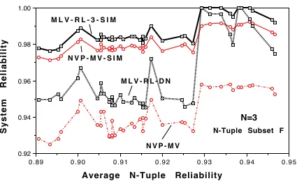
0 . 9 5 0 . 9 4

0 . 9 3 0 . 9 2

0 . 9 1 0 . 9 0

0 . 8 9 0.92 0.94 0.96 0.98 1.00

Average N-Tuple Reliability

System Reliability

M L V - R L - 3 - S I M

N V P - M V - S I M

M L V - R L - D N

N V P - M V

N=3

N-Tuple Subset F

0 . 0 6 0 0 . 0 5 0

0 . 0 4 0 0 . 0 3 0

0 . 0 2 0 0 . 0 1 0

0 . 0 1 0 0.90 0.92 0.94 0.96 0.98 1.00

Standard Deviation of N-Tuple Reliability

System Reliability

M L V - R L - 2

Best Version

Average 3-tuple Reliability

SIMULATION N=3, r=2

N-Tuple Subset F

N V P - M V

Figure 8. Maximum Likelihood Voting compared with Consensus Voting and Majority Voting (system reliability smoothed by symmetrical 11 point moving average, N=3, r=2, and reliability

range from 0.85 to 0.94).

0 . 0 6 0 0 . 0 5 0

0 . 0 4 0 0 . 0 3 0

0 . 0 2 0 0 . 0 1 0

0 . 0 1 0 0.90 0.92 0.94 0.96 0.98 1.00

Standard Deviation of N-Tuple Reliability

System Reliability

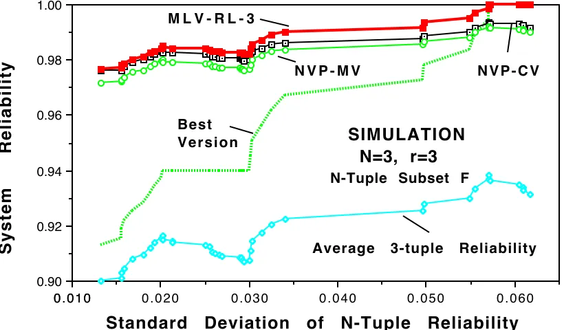
M L V - R L - 3

N V P - M V N V P - C V

Best Version

Average 3-tuple Reliability

SIMULATION N=3, r=3

N-Tuple Subset F

Figure 9. Maximum Likelihood Voting compared with Consensus Voting and Majority Voting (system reliability smoothed by symmetrical 11 point moving average, N=3, r=3, and reliability

range from 0.85 to 0.94).

performance of a strategy, in the same figure we also plot system reliability obtained by simulation under the assumption of no-correlation.

In this simulation, we used exactly the same individual 3-tuple reliabilities as were measured for the Subset F. Each simulated point is an average over 10,000 samples, each sample is the result of a vote done according to the MLV-RL-3 and NVP-MV strategies. In both cases we fixed the simulated output space cardinality to 3. Outputs were chosen randomly and in proportion to their probability of occurrence.

We see that a) simulated MLV performs consistently better than simulated NVP-MV, b) for NVP-MV, there is a significant performance gap between the results expected under conditions of no-correlation (simulation) and the results obtained in our high failure correlation environment (experimental), and c) experimental MLV strategy exhibits a threshold at about 0.93 after which it starts tracking the theoretical performance well.

3.2.3. How system reliability varies with system diversity

The reason N-Version voting, such as Majority or Consensus Voting, has difficulty competing with the "best" version is that the N-tuples of medium to low average reliability are composed of versions which usually are not "balanced", i.e. their reliabilities are very different (diverse), and therefore variance of the average N-tuple reliability is large. This reduces the number of consensus agreements, and this can result in incorrect decisions. The reason MLV does so well, most of the time, is because it is able to select the response based on its performance "history" of the versions that supply it, and thus avoid the voting pitfalls of NVP-CV and NVP-MV that arise from correlated failures. This experimental behavior is in good agreement with the trends indicated by the theoretical Maximum Likelihood Voting model based on failure independence [8]. To gain further understanding of how inter-version correlation and N-tuple diversity interact we revisit Figure 6 through simulation.

confirms this in an indirect way. The performance advantage of MLV over NVP-MV seems to be increasing as the standard deviation of N-tuple reliability increases. Although experiments (Figure 6) show separation of MLV and NVP traces from the very beginning of the range, as the diversity grows the gap in their experimental performance grows too.

Of course, when r=2 Consensus Voting cannot operate [14], so we also simulated the behavior we might expect when r=3, N=3 (the simulated N-tuples again conforming to the individual reliabilities of Subset F). Results are shown in Figure 9. At the low diversity end of the range, the performance of MLV and NVP-CV is almost identical. This is because a) relatively small standard deviation (of N-tuple reliability) means that all individual version reliabilities are almost equal to the average reliability, and b) the lowest average version reliability used in this particular subset is greater than 1/3 (since r=3). As diversity increases, the performance of MLV grows faster than that of NVP. Furthermore, now, in line with empirical observations of Figure 6, the separation in the performance of MLV, NVP-CV and NVP-MV is showing over the whole investigated range.

3.2.4. Exceptions

Unlike Consensus Voting which is always at least as good or better than Majority Voting, MLV is only statistically better than NVP-CV or NVP-MV, and exceptions are possible.

Table 2 provides numerical examples of some of these exceptions. In the table we first show the average reliability of the N-tuple (Avg. Rel.), its standard deviation (Std. Dev.), and the reliability of the acceptance test used in strategies that need it (AT Rel.). The table then shows the average conditional voter decision space (CD-Space), and its standard deviation of the sample. Average conditional voter decision space is defined as the average size of the space (i.e. the number of available unique answers) in which the voter makes decisions given that at least one of the versions has failed. We use CD-Space to focus on the behavior of the voters when failures are present. Of course, the maximum voter decision space for a single test case is N.

We show the count of the number of times the "best" version in an N-tuple was correct (Best Version), and the success frequency under each of the investigated fault-tolerance strategies. Note that MLV data correspond to MLV-RL-DN strategy. The best response is underlined with a full line, while the second best with a broken line. Column 1 (3-tuple), columns 2 and 3 (5-tuple), and columns 4, 5 and 6 (7-tuple) show the cases for the medium reliability versions where NVP-CV performs better than MLV. Columns 7 and 8 (3-tuple) illustrate the same situation for more reliable versions. Column 12 shows the situation where NVP-MV is better than MLV.

(F-Tie). Note that for MLV-RL-DN tie-breaks are quite frequent (section 2.3.4), and only occasionally is the MLV decision based on unique probability maximum (e.g., columns 2 & 11).

In Figure 6, we have shown the results for a more balanced (and higher reliability) set of 3-tuples. The average 3-tuple reliability is not as stable as we would want it to be, but this is because the pool of high-reliability versions was limited. Note that the standard deviations for 3-tuple reliability are an order of magnitude smaller than in Figures 1 through 3. As the version diversity increases, the reliability of Consensus Voting, Majority Voting, and MLV also increases. Again, this is in good agreement with theoretical predictions related to small-diversity (well balanced) version sets.

3.3. MLV VS. Consensus Recovery Block and Recovery Block.

Since MLV appeared to perform very well against "classical" voting strategies, we were very curious to see how it did against an alternative strategy such as the Recovery Block, or against a more advanced strategy such as the Consensus Recovery Block. Theory predicts that, in an ideal situation (version failure independence, zero probability for identical-and-wrong responses), Consensus Recovery Block is always superior to N-Version Programming (given the same version reliabilities and the same voting strategy) [1] or Recovery Block [12, 3] (given the same version and

Table 2. Examples of cases where MLV was less reliable than other strategies.

1 2 3 4 5 6 7 8 9 10 11 12 13 14 15 N-tuple Structure

Subset G1 J 1 J 38

M 4 M 25 M 36 F 20 F 25 F 21 F 32 F 40

I 1 I 49

L 2 L 36 Versions 5,9 ,13 8,9 ,11 ,13 ,17 8,1 0,1 1,1 7,1 9 4,7 ,10 ,11 ,12 ,15 ,17 3,5 ,6, 7,8 ,11 ,13 3,4 ,5, 6,7 ,8, 13 7,1 1,1 7 4,1 1,1 3 7,1 1,1 3 5,1 1,1 7 3,4 ,11 5,7 ,10 ,11 ,17 3,4 ,7, 11, 13 3,4 ,7, 10, 11, 13, 17 3,4 ,7, 8,1 0,1 1,1 3 Mean Value

Avg. Rel. 0.80 0.79 0.77 0.79 0.79 0.79 0.92 0.90 0.91 0.90 0.91 0.93 0.91 0.92 0.88

Std. Dev. 0.16 0.15 0.24 0.26 0.21 0.22 0.02 0.03 0.03 0.00

4 0.02 5 0.04 2 0.02 8 0.04 0.11

AT Rel. 0.93 0.93 0.93 0.93 0.93 0.93 0.93 0.93 0.93 0.93 0.93 0.93 0.93 0.93 0.93

CD-Space 2.13 2.79 2.67 3.31 3.12 3.15 2.12 2.29 2.11 2.17 2.32 2.27 2.47 2.53 2.59

Std. Dev. 0.34 0.70 0.58 0.64 1.17 0.79 0.33 0.46 0.31 0.37 0.47 0.44 0.71 0.93 0.93

Success Frequency

Best Version451 450 500 500 470 470 470 470 470 455 470 500 465 500 500

MLV-RL-DN

454 467 467 482 481 468 486 468 486 451 482 481 482 482 486

NVP-MV 454 450 449 468 442 442 486 468 486 451 466 486 482 482 482

NVP-CV 459 470 475 493 485 473 491 482 489 455 478 494 486 493 493

RB 468 472 476 474 471 467 478 480 482 473 473 476 477 472 478

CRB-MV 468 472 468 474 471 467 492 480 496 467 487 491 491 486 492

CRB-CV 468 469 468 491 484 467 492 480 496 467 487 491 486 490 493

Success Frequency of some MLV Sub-Events

S-Total 454 467 467 482 481 468 486 468 486 451 482 481 482 482 486

F-Total 46 33 33 18 19 32 14 32 14 49 18 19 18 18 14

S-Tie 454 465 467 482 467 467 486 468 486 451 455 481 482 482 486

acceptance test reliabilities). But, there is no theoretical analysis that compares MLV with RB or CRB, particularly not under excessive inter-version failure correlation conditions.

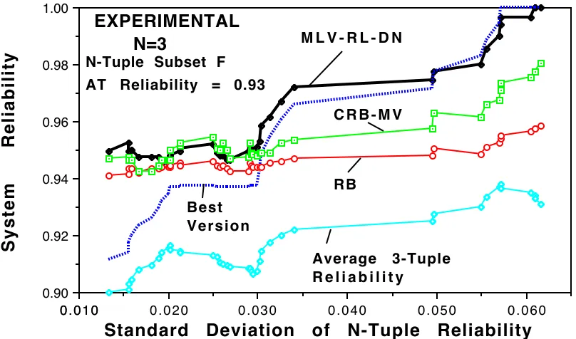
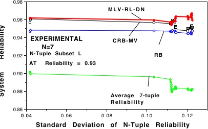
Figure 10 shows the performance of MLV, CRB-MV and RB with a set of relatively well balanced medium to high reliability versions (0.85 to 0.94). The same acceptance test version was used by Consensus Recovery Block and by Recovery Block (reliability of acceptance test is 0.93). From the figure we see that for N=3, reliability of Maximum Likelihood Voting is comparable or better than that of CRB-MV. However, the reliability performance advantage of MLV over CRB diminishes as the N-tuple size increases (see Figures 11 and 12, Table 2 columns 9 to 15). When compared with Recovery Block, MLV tended to perform better than RB over the whole investigated range. On the other hand, while CRB-CV tended to be better than RB, performance of RB was better than CRB-MV for lower reliability versions (Figure 13). Note also that although the reliability of RB is primarily governed by the reliability of its acceptance test, our implementation of RB outperforms its acceptance test by a small margin.

0 . 0 6 0 0 . 0 5 0

0 . 0 4 0 0 . 0 3 0

0 . 0 2 0 0 . 0 1 0

0 . 0 1 0 0.90 0.92 0.94 0.96 0.98 1.00

N-Tuple Subset F

Standard Deviation of N-Tuple Reliability

System Reliability

EXPERIMENTAL N=3

Average 3-Tuple R e l i a b i l i t y

RB C R B - M V

Best Version

M L V - R L - D N

AT Reliability = 0.93

Figure 10. MLV compared with CRB-MV and RB (system reliability smoothed by

0 . 0 4 7 0 . 0 3 7

0 . 0 2 7 0 . 0 1 7

0 . 0 1 7 0.90 0.92 0.94 0.96 0.98 1.00

N-Tuple Subset I

Standard Deviation of N-Tuple Reliability

System Reliability

EXPERIMENTAL N=5

AT Reliability = 0.93 Average 5-tuple

R e l i a b i l i t y

RB C R B - M V

M L V - R L - D N Best Version

Figure 11. MLV compared with CRB-MV and RB (system reliability smoothed by

symmetrical 11 point moving average, N=5, and reliability range from 0.85 to 0.94)

0 . 1 2 0 . 1 0

0 . 0 8 0 . 0 6

0 . 0 4 0 . 0 4 0.86 0.88 0.90 0.92 0.94 0.96 0.98

N-Tuple Subset L

Standard Deviation of N-Tuple Reliability

System Reliability Average 7-tuple

R e l i a b i l i t y

EXPERIMENTAL N=7

AT Reliability = 0.93

M L V - R L - D N

RB C R B - M V

Figure 12. MLV compared with CRB-MV and RB (system reliability smoothed by

3 . 2 4 3 . 1 4

3 . 0 4 2 . 9 4

2 . 8 4 0.930 0.940 0.950 0.960

0.970 EXPERIMENTAL

N=7

Average Conditional Voter Decision Space

System Reliability

N-Tuple Subset M AT Reliability = 0.93

M L V - R L - D N

C R B - M V RB

CRB-CV

Figure 13. Voter behavior in small decision space (system reliability smoothed by symmetrical 11 point moving average, N=7, and reliability range from 0.70 to 0.79)

3.3.1. What is the influence of the effective decision space

The final thing we want to highlight is the influence of the effective output space, specifically of the CD-Space. To illustrate the relationship between the voter decision space cardinality and the performance of MLV we plotted (in Figure 13) the system reliability of MLV, CRB-CV, CRB-MV and RB against the average conditional voter decision space. The average conditional voter decision space was calculated as the mean number of distinct results available to a voter during events where at least one of the 7-tuple versions has failed. Note that in Figure 13, the variation in the voter decision space size is caused by the variation in the probability of obtaining coincident, but different, incorrect answers. As the decision space increases, the reliability of Maximum Likelihood Voting appears to increase at a faster rate than that of the Consensus Recovery Block strategy, and by implication faster than that of NVP-CV or NVP-MV. This behavior is in good agreement with theory [8].

4. Summary and conclusions

MLV carries only statistical and not absolute guarantees, the advantage of MLV is that in most situations its performance is consistently better than that of Consensus Voting or Majority Voting. This is especially true when average N-tuple reliability is low and/or standard deviation of N-tuple reliability is high.

A practical disadvantage of Maximum Likelihood Voting comes from the added decision complexity, and the additional testing effort needed to get a good independent estimate of operational version reliabilities. When compared to Consensus Recovery Block and Recovery Block, MLV performance competes well, and MLV even appears to be more stable and robust in some situations. The effectiveness of MLV significantly increases as the version diversity increases or the voter decision space increases. In general, our experimental results agree well with the behavior expected on the basis of the analytical studies of MLV made by Leung [8].

Of course, behavior of an individual practical system can deviate considerably from that based on its theoretical model average so considerable caution is needed when predicting behavior of practical fault-tolerant software systems, particularly if presence of inter-version failure correlation is suspected. For example, while our results seem to confirm the theoretical superiority of MLV over Consensus Voting and Majority Voting in a statistical sense, they also demonstrate that in real situations there are exceptions where MLV may not perform better than NVP-CV or even NVP-MV. This raises some safety concerns when it comes to possible use of MLV in life-critical applications.

REFERENCES

[1] A.M. Athavale, "Performance Evaluation of Hybrid Voting Schemes", M.S. Thesis, North Carolina State University, Department of Computer Science, 1989.

[2] A. Avizienis and L. Chen, "On the Implementation of N-version Programming for Software Fault-Tolerance During Program Execution", Proc. COMPSAC 77, pp 149-155, 1977. [3] F. Belli and P. Jedrzejowicz, "Fault-Tolerant Programs and Their Reliability", IEEE Trans.

Rel., Vol. 29(2), pp 184-192, 1990.

[4] A.K. Deb, and A.L. Goel, "Model for Execution Time Behavior of a Recovery Block", Proc. COMPSAC 86, pp. 497-502, 1986.

[5] D.E. Eckhardt, A.K. Caglayan, J.P.J. Kelly, J.C. Knight, L.D. Lee, D.F. McAllister, and M.A. Vouk, "An Experimental Evaluation of Software Redundancy as a Strategy for Improving Reliability", IEEE Trans. Soft. Eng., Vol. 17(7), pp 692-702, 1991.

[6] J. Kelly, D. Eckhardt, A. Caglayan, J. Knight, D. McAllister, M. Vouk, "A Large Scale Second Generation Experiment in Multi-Version Software: Description and Early Results", Proc. FTCS 18, pp 9-14, June 1988.

[7] J.C. Knight and N.G. Leveson, "An Experimental Evaluation of the assumption of Independence in Multi-version Programming", IEEE Trans. Soft. Eng., Vol. SE-12(1), 96-109, 1986.

[8] Y.W. Leung, "Maximum Likelihood Voting for Fault Tolerant Software with Finite Output Space", IEEE Trans. Rel, Vol. 44(3) pp 419-427, 1995

[9] D.F., McAllister, C.E., Sun, M.A, Vouk, "Reliability of Voting in Fault-Tolerant Software Systems for Small Output-Spaces", IEEE Trans. Rel, Vol. 39 (5) pp 524-534, 1990.

[11] R.K. Scott, J.W. Gault, D.F. McAllister and J. Wiggs, "Experimental Validation of Six Fault-Tolerant Software Reliability Models", IEEE FTCS 14,1984

[12] R.K. Scott, J.W. Gault and D.F. McAllister, "Fault-Tolerant Software Reliability Modeling", IEEE Trans. Software Eng., Vol SE-13, 582-592, 1987.

[13] M.A., Vouk, A., Caglayan, D.E., Eckhardt, J., Kelly, J., Knight, D.F., McAllister, L., Walker, "Analysis of faults detected in a large-scale multiversion software development experiment", Proc. DASC '90, pp 378-385, 1990.

[14] M.A., Vouk, D.F., McAllister, D.E., Eckhardt, K., Kim, "An Empirical Evaluation of Consensus Voting and Consensus Recovery Block Reliability in the presence of Failure Correlation", JCSE, 1(4), pp 364-388, 1993.

[15] K. Kim, M.A. Vouk, and D.F. McAllister, "An Empirical Evaluation of Maximum Likelihood Voting in Failure Correlation Conditions," Proc. ISSRE 96, pp 330-339, 1996 [16] D.E. Eckhardt, Jr. and L.D. Lee, "A Theoretical Basis for the Analysis of Multi-version

Software Subject to Coincident Errors", IEEE Trans. Soft. Eng., Vol. SE-11(12), 1511-1517, 1985.

[17] B. Littlewood and D.R. Miller, "Conceptual Modeling of Coincident Failures in Multiversion Software," IEEE Trans. Soft. Eng., Vol. 15(12), 1596-1614, 1989.

[18] M.R. Lyu (ed.), Software Fault Tolerance, Wiley Trends in Software book series, John Wiley & Sons, 1995.

[19] M.R. Lyu (ed.), Handbook of Software Reliability Engineering, McGraw-Hill and IEEE Computer Society Press, New York, 1996.

APPENDIX I: INTER-VERSION FAILURE CORRELATION

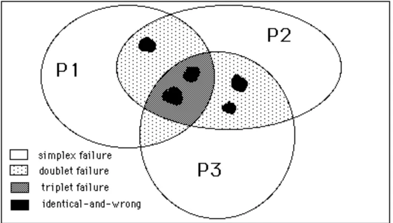
We use the terms "coincident", "correlated" and "dependent" failures (faults) with the following meaning. When two or more functionally equivalent software components fail on the same input case we say that a coincident failure has occurred. Failure of k components raises a level-k coincident failure. The fault(s) that cause a level-k failure we shall call level-k fault(s). When two or more versions give the same incorrect response (to a given tolerance) we say that an identical-and-wrong (IAW) answer was obtained. If the measured probability of the coincident failures is significantly different from what would be expected by random chance, usually based on the measured failure probabilities of the participating components, then we say that the observed coincident failures are correlated. Note that two events can be correlated because they directly

depend on each other, or because they both depend on some other, but same, event(s) ( indirect

dependence ), or both.

Let Pr{ } denote probability. Then

Pr{ version(i) fails | version(j) fails } ≠ Pr{ version(i) fails } (A1.1) means that the conditional probability that version "i" fails given that version "j" has failed is different from the probability that version "i", considered on its own, fails on the same inputs. If this relationship is true, we do not have failure independence [20].

We say that several components contain the same or similar fault or common-cause fault if the fault's nature, and the variables and function(s) it affects, are the same for all the involved components. The result (answer) of execution of common-cause faults may be identical (IAW to within tolerance), or may be different. It is also possible that different faults result in a coincident failure by chance, giving either different answers or IAW answers.

Figure A1.1 Venn diagram of the failure space for three hypothetical functionally equivalent programs.

Possible failure events are illustrated in Figure A1.1. The Venn diagram shown in the figure4 represents the overlaps in the failure space of three functionally equivalent software units (or a

3-tuple of variants). Unshaded areas are regions where one of the three components (programs: P₁, P₂, P₃) fails for an input. Lightly shaded areas show the regions where two out of three components fail coincidentally, while the darkly shaded area in the middle is the region show where all three components fail coincidentally.

Of special interest are regions marked in black which represent events where components produce IAW responses. Any failures that occur in these regions are unsafe since the voting algorithm has no way of telling that a failure has occurred in the first place. Failures in the other regions may be called safe in the sense that the disagreement among the version outputs offers an indication that a failure may occur (if voting is undertaken) and it is possible to warn the user of that if the designer of the voter wishes to do so.

APPENDIX II: VOTING STRATEGIES

Majority Voting (NVP-MV) chooses the majority agreement output as the correct answer and it reports a failure if there is no majority agreement.

Consensus Voting (NVP-CV) chooses a maximum agreement (not necessarily a majority) as

the correct answer.

In Recovery Block (RB), versions are ranked, the "best" version is executed and its output is tested for acceptance. If the output fails the acceptance test, the "next best version" is executed, etc., until an acceptable answer is obtained. If all versions fail acceptance test, an error is reported.

The Consensus Recovery Block (CRB) is a hybrid strategy which combines both Recovery

Block and N-Version Programming (either NVP-CV or NVP-MV). When CRB is invoked, it begins operating in an N-Version Programming mode. All versions are executed and a vote is executed. If voting fails, CRB enters Recovery Block mode. [12] If the Majority Voting is used in the N-Version Programming mode of CRB, we call it CRB-MV. If the Consensus Voting is used, it is called CRB-CV. [14]

APPENDIX III: THE MLV-RL-DNALGORITHM

The Maximum Likelihood Voting (MLV) implementation based on tie-breaking that uses version reliability estimates is described in the following pseudo code:

function Maximum_Likelihood_Voting() real Likelihood[1..N+1];

set MaxVersion; {

/* Compute likelihood values for each version using the formula (see equation (3)) */

for i = 1 to N+1 Likelihood[i]=

compute_likelihood(i);

/* Identify the values for Maximum Likelihood and remember it. */ MaxLikelihood =

find_max_likelihood(Likelihood,N+1);

/* Identify any version outputs whose likelihood is equal to Maximum value identified in previous step */

for i = 1 to N+1

if (abs(Likelihood[i]-MaxLikelihood) < tolerance)

{

likelihood values */ MaxVersion.add(i); }

/* More than 1 versions have same maximum likelihood values */ if (MaxVersion.card() > 1)

{

/* Choose the version with the largest reliability estimate among these ties.*/ return

MaxVersion.getMaxMostReliable(); }

else {

/* Only 1 version has the highest maximum likelihood value, choose this version as a correct answer. */

return MaxVersion.getMax(); }

}/* Maximum_likelihood_Voting() */

Note that the program above calculates likelihood values N+1 times (N possible realized outputs and 1 unrealized output representing entire unrealized outputs), where N is the number of versions used in voting.

APPENDIX IV: SELECTION OF N-TUPLES

To select subsets of N-tuples which have certain properties such as approximately equal reliabilities we used the following approach.

We first select acceptance test versions based on Estimate I data (for example, one low reliability, one medium and one high reliability acceptance test). These versions are then removed from the pool of 20 versions. For a given N the remainder of the versions (a subpool that now has 17 versions) are then randomly sampled without replacement. The average N-tuple reliability is then computed, and if it lies within the desired reliability range the N-tuple becomes a member of the subset. Then the N-tuple versions are returned to the subpool and the next N-tuple is selected in a similar manner, etc. Once the subset contains either all possible combinations, or at least 1000 N-tuples (whichever comes first), the subset is sorted by the average N-tuple reliability and then the first 50 versions are chosen and run in the experiment.

We have thus selected a number of subsets. The following are mentioned in the text

N-Tuple Subset F : 3 version systems, average 3-tuple reliability in the range 0.85 to 0.94, acceptance test reliabilities of 0.67 (version 20), 0.93 (version 2) and 0.994 (version 18).

N-Tuple Subset G : 3 version systems, average 3-tuple reliability in the range 0.70 to 0.79, acceptance test reliabilities of 0.67 (version 20), 0.93 (version 2) and 0.994 (version 18).

N-Tuple Subset H : 3 version systems, average 3-tuple reliability in the range 0.55 to 0.64, acceptance test reliabilities of 0.67 (version 20), 0.93 (version 2) and 0.994 (version 18).

N-Tuple Subset I , 5 version systems, average 5-tuple reliability in the range 0.85 to 0.94, acceptance test reliabilities of 0.67 (version 20), 0.93 (version 2) and 0.994 (version 18).

N-Tuple Subset J , 5 version systems, average 5-tuple reliability in the range 0.70 to 0.79, acceptance test reliabilities of 0.67 (version 20), 0.93 (version 2) and 0.994 (version 18).

N-Tuple Subset L , 7 version systems, average 7-tuple reliability in the range 0.85 to 0.94, acceptance test reliabilities of 0.67 (version 20), 0.93 (version 2) and 0.994 (version 18).

N-Tuple Subset M , 7 version systems, average 7-tuple reliability in the range 0.70 to 0.79, acceptance test reliabilities of 0.67 (version 20), 0.93 (version 2) and 0.994 (version 18).