A review of nest survival models

Cooperative WUdute and Fisheries Statistics Project Department of Statistic., North Carolina State University

Box 8203, Raleigh, North Carolina 27695-8203

ABSTRACT

In manT nest survival studies nests are not found until after incubation has belr\1n, and nests which fail are of unknown age while nests which succeed can be aged afterward. Originally ornithologists ignored all these problems and just reported the fraction of nests which were successful

(Naive Approach). Now, tTPica1ly, ornithologists consider the survival time to be from first encounter, and they use what has come to be known as the MaTfield method (Mayfield 1961, 1975) or some variation

ot

it. Pollock (1984)

e

and Pollock and Cornelius (in prep.) considered a new approach which allows

estimation of the survival distribution from the time

ot

nest initiation, which is the actual time origin. Nests which succeed are used to estimate the proportions of nests being found (encountered) in each time interval. Assuming that these encounter probabilities also apply to the nests which fail, it is possible to estimate a serie.

ot

discrete failure time probabilities for all the nests. Here we review the models and assumptions for the Naive approach, the Mayfield method and the Pollock method. We compare estimates and their precision. We also explore the ditterences between the modeling of nest survival and egg survival.

1. INTRODUCTION

Nesting survival studies are those in which an ornithologist chooses a

_stud)" area and searches for active nests to observe. Nests found are visited

regularly until the)" are either abandoned or deetro78d, or until the)"

produce )"oung birds which hatch and later fledge. For any given species, it

is generally accepted that the number of days from egg initiation to hatching

(incubation) is approximatel)" constant, and the number of da)"s from hatching

until fledging is again approximately constant. In these 2 intervals of time, the nest and its )"oung are at risk to such perils as predator pressure, lack

of availability of food, bad weather and others.

In many nest survival studies nests are not found until after incubation

has begun; and nests which fail are. of unknown age, while nests which

e

succeed can be aged afterwards. Three distinct methodologies or models have served to describe this special kind of data and are to be reviewed in

this article.

In Section 2 we consider the Naive approach originally considered by ornithologists. With t.his method aU the special aspects of the data are

iarnored and simply the fraction of nests which are successful is reported.

In Section 3 we consider the the Ma)"field method. In Mayfield (1961,

1975) the survival time from first encounter is considered. This enables one

to find the total number of nest da)"s of exposure and this together with the

number of failures enables one to obtain a dail7 survival rate. In Section 4

•

In Section 5 we review a new approach (Pollock 1984; Pollock and

Cornelius in prep.) which allows estimation of the survival distributions from the time of nest initiation which is the natural time oriain. Nests which succeed are used to estimate the proportions of nests found (encountered) in each time interval. Assuming that these encounter probabilities also apply to the nests which fail it is possible to estimate a series of discrete failure time probabilities for all the nests. In Section 6 a detailed comparison of the three approaches is made using some mourning dove data and then using some Great-Tailed Grackle data.

Nest success is defined as survival of one or more eggs in a nest until the young have fledged. The paper concludes with a general discussion section.

2. NAIVE SYCCESS ESTIMATES

In the earliest studies of nesUn.'8\lCCeSS, it was customary to report one's findings by giving the numbers of nest.- and eggs in the sample, the

number of eggs that hatch, number of 10ung birds fledged and various derived percentages. Mayfield (1961) described this practice, without citing examples of it.

e.

from this is that

ot

all dove nests established in the wild, 25/59 or 42.4% will 7ield new birds, (std. error

=

6.4%), in accordance with binomial distribution

theory.

The first difficulty with this approach i. a .. kind of sampling bias

problem. We make use of a sample of discovered nests to make inference for

a population of concealed nests, assuming the sample to be randomly selected

from the population. But even when this method was practiced, field workers

would find and take data from every nest they possibly could, simply

because of the great difficulty of finding a satisfactory number of nests to

report on.

Unhatched nests encountered in the wild will be

ot

various unknown ages, 1, 2, ..., J days, where J is tM. incubation period for the species. Nests near J days of age have a higher probability of survival than nests near 1 day of age. Yet in the procedure Juat ou.tlined, the average survival

observed ·was taken to be the avera... survival of all nests initiated in the

wild. All nests are initiated at age 1, not at 80m. distribution

ot

ages from 1 through J.

This sampling was not unknown or as unappreciated by field workers as .

our discussion might imply. Presumably, training and experience gained by

field workers can help them become better able to find many nests in the

first few days

ot

incubation. This will result in samples that are more nearly representative of the population. Bias in the estimator can also be reduced

in this case by consideration

ot

the data. Once nest eggs hatch, the age of the nest becomes known; those nests not found early in the incubation period

ot

the nest when first found remains unknown, but a well-trained field

worker can estimate it fair17 accurate17 an;ywa7, 80 that tailing nests too old

•

constant for all daY's in the incubation cY'cle. If the dailY' survival rate is

PDAIU, then the interval survival rate (correspondina to the Naive p) is

PDAIL1'7, where J is the number

ot

days in the incubation period.

A areat advantage gained by Mayfield's method is the ability to make use

of almost all the data collected in the field. AnY' viable nest that is observed

on 2 difterent days can be included in the calculations. Another advantage

is that there is less demand for inclusion of nests found near the beginnina

of the incubation cycle; all days in the cycle are equally valuable.

To illustrate the Mayfield method, let us again consider the dataset

analyzed by Nichols et al. (1984).

.

There were 59 nests, with 25 hatching and. .

34 failing, but now we will note that the hatchina nests were observed to occur 11 after 1

.

to

8 days, 8 more alter 9

to

16 days, and 6 after 17 or more

.

days; while the failing nests failed 16 within tJ1e first 8 days, 9 within the

next. 8, and 9 within the .final 10 of 26 days (some

ot

these may be nestling deaths rather than all egg deaths). Thus the nests which hatched account

tor 11 x 8

+

8 x 16

+

6 x 26

=

312 nest-days, and the nests which failed

account tor 16 x 8 x 0.5

+

9 x (8

+

8 x 0.5)

+

9 x 10 x (16

+

10 x 0.5)

=

361

nest-days. In such a study, where nests are not observed every day, the

eJt8Ct day a nest tailed would not be known, so Mayfield suggested that the

midpoint between the observations be used, hence the "0.5" values given

here. In tact the nests in this example were observed daily, 80 the number

of nest-days is known exactly, without recourse to estimating that all

Buccesstul nests hatched at the endpoin.ts

ot

8 or 10 day intervals and that

·e

accounted tor 386 and 324 nest-da)"s, respectively. There were 34 falling

nests in 710 nest-da)"s of data, whence qOAJ:LY

=

34 I 710

=

0.04789, PDAJ:LY

=

0.9621 (std. error

=

0.008014); p

=

PDAJU"

=

0.2792 (std. error

=

0.0610).

Ma)"field (1975) ar&,ued the case that. survival rate is unlikely to be

constant from da)" to da)", though he continued to advocate assuming this on

the arounds that the usual nesting stud)" failed to obtain sufficient. data to

make differing dail)" estimates, and the dail)" rate might not vary so seriousl)"

as to require differing rates. He did suggest attempting to determine

different rates for hatching and fledging, and he proposed applying a

Chi-Square test of the difference bet.ween these.

4. EXTENSIONS TO THE MAYFIELD METHOD

If nests are not observed on a dail)" basis, Ma)"tieldproposed that nests

• found to fail be assumed to have tailed in the cepter

ot

the unobserved period. This actuall)" is in deffe.nce of" the constant dail)" survival rate

IJSsumption: it is a linear rather than aaeometric decrease.

Miller and Johnson (1978) gave apparenU7 the first published critique of

this assumption. The7 proposed that when da7. are skipped between nest .

visits and failure is subsequentl7 observed, then not the mid-point, but the

40% point should be assigned as the 97 of failure.

Johnson (1979) compared the performance of the ori~nal Ma)"field

estimator (50%), his and Miller's "Mayfleld-40X" method, and a third method in

which the failure assianment is made b7 maximizing the likelihood of the

Jla7f1eld model. Johnson (1979) also first published variance estimates for

the estimator, b7 deriving the estimator as a maximum likelihood estimate

••

sample variance (from t.he maximum likelihood information matrix). He t.hen

compared the 3 interpolation methods on some datasets and concluded that

the differences in results were not substantial, and t.herefore in man,. cases

the original Mayfield method is acceptable and the easiest one to use; one of

the other methods ma,. be sil'nificantl,. better if the int.erval between nest

visits is ver,. long.

Using Mayfield's nesting model, Hensler and Nichols (1981) again showed that his proposed estimator is a maximum likelihood estimator. The,.

calculated its as,.mptotic distribution and proposed an estimator of the

8871DPtotfc variance. From this the,. derived confidence intervals and tests

of significance for dail,. survival. The,. performed extensive Monte Carlo

simulation to determine the performance of the estimators and tests under

man,. different sets of conditions. The,. showed the Naive estimator of

nesting success to be "quite interior to the Mayfield estimator. The,. gave

sample size requirements to achieve set level~ of accurac,. for their tests.

Bart and Robson (1982) did a thoroui'h job

ot

characterizing the

samplinl' distribution of the Ma1field method(s), showinl', for example, that its

normalit,. could be improved b,. means

ot

a square root transformat.ion. The,.

obtained a sampling distribution close

to

that of Johnson. The,. also developed distributions of differences between 2 rates and products of 2

rates (sa,. an earl,. rate and a late rate are thoul'ht to be different .and beg

testinl', but the net. over-all rate remains the focu8 of the researcher's

interest (p

=

PUUyz-- PLATE-

=

PDAXU Z

».

Hensler (1985) proposed applying

the Mayfield method "piecewise" to this type

at

problem and showed how to

•

.MaTtield's implicit assumption that all nests have the same daily rate(s)

at

aurvival was challenged bY' Green (1977). The argument was essentiallY'

that density-dependent mortalitY' rates are sometimes observed, and if so, they are a manifestation of heterogeneitY'i in particular, "novice~ nesters are less successful than "experienced" nesters. Johnson (1979) presented a

mcdification of the method to expose heterogeneitY' and adjust for it. The

procedure employed was to age the nests and compute daily mortality rates

by age of nest, compute a regression line through these data and accept the

intercept of this line as the success rate, instead of the rate that comes from

thtt lltandard MaTtieid method with the pooled data. Based on some data,

Johnson declared that MaTtield's method seems to be quite robust to

hetero,~neitY'•

An assumption acknowledged bl' Ma)"fleld (1975) is that the samplin, process doe, not perturb the success rates. MaTtieid preferred a daill'

obattrvation period, but noted that some ob. .rv.rs believe that visitin, a

nest toQ frequentlY' imparta greater mortalit,. to it. His method does not require daily visits. Some field workers have adopted the custom of being in

the field ever,. da,., but visiting a nest onI,., sa,., once a week so long as

distant observation of the nest su.gesta it i8 still succeedingj if the distant obattrvation casts doubt on successfulnes8 of the nest thel' mal' make an

1UUICheduied visit in order to document accuratel,. the time of failure. It the

act of visiting increases the probability of failure, this is certainly a biasing

procedure. Bart and Robson (1982) also proposed extensions of the model for

var7ing survival rates and for visitor-induced depression of survival,

•

out that it is not necessary to visit nests daily, nor at any certain fixed interval. Visiting intervals may vary systematically or randomly. It is,

however, necessary to avoid using the field worker's belief about the current tate

ot

the nest to decide when to visit.

5. THE POLLOCK METHOD

Pollock (1984) and Pollock and Cornelius (in prep.) offered a new discrete survival model allowing estimation of the survival distribution from the time of nest initiation, a more natural time origin, rather than from time of first encounter as used by all the earUermodels. They also abandoned the assumption that survival events (nest days) need have constant probability.

Pollock's method was the first to model nestin&, survival intentionally from the first day of the nest. This is done by usin&, the observed age distribution of successful nests to inter the unobservable age distribution of failing nests. Survival probabilities can be conditioned on this distribution.

(Earlier models could roughly accomplish the same result only if their failing nests were found on the first day with very hiah probability, and on later days with close to zero probability.) There is no constant probability assumption in this model because each day-or-event probability is estimated separately, without constraint, independently

ot

the others.

Model Structure

This model uses a discrete distribution free approach. We denote the age at death or successful termination

ot

the ith nest as Ti. This random

•

Model Par8JDeters

The model encOJlPuses a set of nest failure probability Parameters and a

set of encounter probability parameters. The failure Par8JDeters are

ql

=

P(T

=

1)i ~

=

P(T

=

2)i ... i qJ'

=

P(T

=

J')

where qj is the probability a nest is found failed at age j although it was successful to age j-l. The q.'s are unconditional probabilities of failure,

. J

and therefore the probability of a nest succeeding is

P

=

I - ql - ~ - ••• - qJ'. There are J' distinct failure Parameters in the

aodel. The age units could be days, two days, weeks or whatever is JIOst appropriate. In fact, it ia not even necessary that the age intevals be

equal.

The encounter ~ers are a set of J' nuisance p8r8JDeters

cSl' cS₂' .... ' cSJ' where cSj is the probability of an intact nest ~eing first encountered at age j (swIer to 8₁,

'2' ...

8J' of Hensler and Nichols

(1981».

A critical assUIIPtiOD of the Pollock 1IOde1 is that these encounter

probabilities are independent of the survival probabilities given above. In

other worda, nests encountered early or late in the cycle are not JIOre or less

likely to survive future time units.

Data Available

Application of the Pollock JIOdel entails tabulating the number of

D

IB, D2B, ••• , DJH, where

njB isJ the Dumber of nests found of age j which later succeed, and

nu

=

j~lDjB is the total number of successful nests encountered.

Failed nests are denoted n

lF, n2F, ••• , DJF, where

njF is the number of Dests of unknown age which are observed for j units of time and then fail.

J

nF

=

j~lnjF is the total number of unsuccessful nests eDcountered. Pollock and Cornelius (in prep.) analyzed the likelihood as the product of three conditional multinomial distributions

(i) _{P (nIH' n2H, ••• ,} nJHI~) the conditional distribution of the • Dumbers of successful nests of each age at encounter (njB j = 1, 2, ••• , J)

given the total Dumber of successful nests (nu)i

(ii) P (D_lF, n_2F, ••• , DJF'D_F the conditional distribution of the Dumbers of Dests of unknown age which fail after i Units of time (njF j = 1, 2, ••• , J) given the total number of nests which fail (D

F); and

(iii) P

(nu'nu

+ D_F) the conditional distribution of the number of successful Dests encountered at any time (nu) given the total number of nests encountered (nu + n

F)·

The encounter parameters are estimated by maxt.izing the likelihood of (i). The resulting estimators are

They are simply the proportions of nests found first in the indicated'

intervals. Failure paralleters are estillated by l18Ximizing the likelihood of

(ii) aDd (iii) and substituting the

6

j .tiJlates fOUDd frOil (i) for the 6j factors here. These equations are

(6

1 ql

+

6

2

~ + ••• +

6

J qJ)

I

D

=

nl

F In

r

(6

₁

~

+

6

₂

qs

+ ••• +

6

_J-l

q

J)

I

D

=

n₂

,1o,

•

where

•••

3 • J •

(1 -J;l qJ)

I

[(1 -Jil qJ)

+

D)

=

nu

I

(nu

+

o,)

D

=

6

₁ ql +

(6

₁ +

6

2) q2 + ••• +

(6

1 +

6

2 + ••• +

6

J) qJ •

Of these J

.

+ 1 linear equations only J are ind.epeDdent._. Any 1 of the 1st

.3 equations may be elillinated and the rest simultaneously solved for

Bxa!Dle

The following analysis is of lIOUnlinC dove (Zenaida macroura) nest data recorded in 1979 and 1980 at PatuxeDt Wildlife Research Station, Laurel,

Maryland by Jemes D. Nichols. These data bave also been analyzed by Nichols

et al (1984) and Hensler (1985) and were used to illustrate the Naive and Mayfield approaches earlier.

Field workers located 59 (n

=

1Is+ o,) nests containing 1 or 2 eggs each; 34 (o,) of the nests failed to produce fledglings, 16 (n

1,) of those within 8

clays of discovery, 9 (n_2F) within 9 to 16 days after discovery, and 9 (nSF)

of thes~. 11 (nIB) were Dest. first fOUDd DO IIOre thaD 8 days after the eggs

were laid. 8 CDzI) were found wileD eggs were 9 to 16 days old. aDd the r!BlliniDg 6 CD

3B) were found in the D_ting stage <at least 17 days old). The Pollock Model Bst~es

IDcouDter probability est~tes for this ex.-ple are

;1 • ntBfna

=

11/25

=

0.44

<s.e.

=

0.0993)

;2

=

n2Bfna

=

8/25

=

0.32

<a.e.

=

0.0938)

;3

=

~na

=

6/25

=

0.24

Ca.e.

=

0.0854)

Asa~iated failure probabilities are

ql

=

0.29

Cs.e.

=

0.1382)

~

=

0.08

Ca.e.

=

0.1442)

~.

q3

=

0.28

<a.e.

=

0.1104)

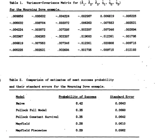
The _YllPtotic variaDce-covariance _trix of the

f

and 9 vectors ia giveD in

Table 1. Notice that while the atandard errors are large. there ia SOllIe

evidence that the failure probabiliti_ are" DOt CODStaDt over the DestiDg

period. In the first 8 days of 1Dcubatiou the failure probability ia high

(ql

=

0.29).

This Jlight be attributed to predatorsfiDdiDg it easy to locate nests and nests of iDexperieDCed breeders being abandoned. In the

aeccmd 8 days of incubation the failure probebility ia IIUCh lower <~

=

0.08).

In the

10

days of nestlings the failure probability appears to riae again

(~

• 0.28).

Thia llight be attributed to predators beine attracted to the

•

- Procr-

SURVIV (White 1983) is useful for this estimation problem, if

iDput specifications are properly

_de,

and especially if the par8lBeter J is

.-11.

The 3 likelihood ca.poneDt syst_ of equations are expressed for SURVIV as 3 "cohorts" in the P&OC ~DBL specification of progi'811 SURVIV•. lor our example, the input to SURVIV should appear • in Figure 1.

(ODly 2 J - 1 equationa need to be specified, because the COHOin'

cell probabilities always 8UII to 1, and SURVIV by default creates en

edditional cell in each cohort whose probability is .signed the difference betweD 1 and the s . o't the other, explicit cell probabilities. This_8D8 tbat one o't the J eqiJatiOD1l in each o't the 1st 2 COHORTs C8D be dropped frOll

the specification. We c:.itted the equation defiDing 6

3; we introduced it

GDCe in the 2nd COBOIn' . . the expression I - 6₁ - 6₂.)

The probability of a nest succeeclinc is giveD by

P

=

1 - ql-:

~-

q3

=

0.35 with a stendard error of 0.0660. This eatmat. is web more precise then the iDdividual q estimates because of the -eati". covari:ences between the ~'s (Table 1).

The flexibility ofPrograa suavIV is extr_Iy useful. In Figure 2, this

aecoDd set of code deJlODstrates iJIpositiou of • COIHItent survivorship

-..ptioD (ql

=

q, ~

=

(l-q)q, ~ • (l-q) (l-q)q). The result obtained

is that the const8Dt (conditional) probebility of failure at each stage is

0.29 with stendard error 0.0428. The probability of a nest succeeding is

pven

by

P

=

(1~3

== 0.3S with a sttlDdard error of 0.0642. A likelihood ratio teat of the reduced versus the full JIOdel is easily obtained

•

•

ADother ccmputer prograa to solve this estiJlation problem, NESTING, is

available fro. the authors. Our progr&ll caD haDdle larger failure vectors thaD SURVIV. NESTING solves the likelihood equatioDs explicitly for point

_ti_tes· and us_ sbulation for variance estiJlates, while SURVIV uses a

quasi-Newton m-erical optiJaization algorithll (Kennedy and Gentle 1980, pp. 461-460)

to

obtain all estiJlates.

Model AssUllptions

The first .sUllptioa of the Pollock lIOdel is that the nests observed coutitute a nmdoa .-pIe with re8pect to survival. This s _ asau.ption is

required of all .-pliDg procedures to esti.Dlate survival rates (radio-tagging

_thod,

capture-recapture met1?-od). If .the nests which are easier to find also

have higher predation rat_ it could be violated.

There is DO seasonal cc.poDeDt in this 1IOde1. All nests are treated as

a cohort

trOJI

time of initiation. If the . . . .le were large enough one could str.atify the HllPle into early, -.di. and late nests and =-pare the aurvival diatributioas. ADother pouibility 18

to

treat calendar time as • covariate and build a relatioaship directly into the -:Miel. '!'his needs

fUrther investigation.

'!'his -:Hiel requires the assUliption that visiting the nest does not iDtlueuce its survival. Bart aDd Robsoa (1982) state that, "In SOlIe cases,

riaitiDg the subject -.y tellPOrarily depress its cbaDce of survival.

observers .ay leed predators to the DeSt or cause nest abandoDIIeDt". They present aD extension of the Mayfield t~ -:Hiel to allow a tellPOrary visitor

•

also emphasized the importance of a regular schedule of visits (daily,

weekly). SaaetiJles biologists are tempted to change the schedule if they.

thiDk a nest is just about to fail.

The lIOdel assUIIPtions meDtioned above are also required by the traditional Mayfield Method. In addition the Mayfield Method requires the assUIIIPtion of

constant survival per time-unit; however in some cases the Mayfield is applied

separately to segllleDts of the nesting period to weaken this assUIIIPtion.

A very critical assUIIIPtion to this DIOdel is that encounter probabilities

are not related to the subsequent success of nests. For exsaple, nests

encountered close to the beginning of the nesting cycle iDay hapPeD to be

highly visible and accordingly more likely to suffer predation than older

nests. This assUJDption will need to be investiga~edin more detail using

siJllulatioD'•

6. A COMPARISON OF THE MODELS

Mourning Dove Example

ID 'fable 2 we compare the probability of nest success estimates and their standard errors for the Naive Model (lIw'n), the Pollock Full Model,

the Pollock Constant Survival Model, the Mayfield Model and the Mayfield

Model calculated for each period separately as we have applied thea to

the Nichols et ale (1984) data. Both Mayfield estimates are calculated on a

daily buis. We find the results on precision soaewha.t surprising. IDtuition

suggests that the more parBDleters that JlUSt be estimated, the poorer the

precision that will result; Pollock estimates should be rather imprecise. But

the realized precisions of both Pollock estimates are almost identical to

•

Although the Pollock model estimates more parameter values, it makes use of

IIOre information than the Mayfield Model. The Pollock estimates are about

midway between the Naive estimate (0.42), which is known to be positively biased, and the Mayfield estimate (0.28). If the standard errors are

considered, neither Pollock estimate is significantly different from either

Mayfield estimate.

Great-Tailed Grackle Example

We now compare the models using some Great-Tailed Grackle (Quiscalus

mexicanus) data collected by Scott Winterstein near Los Cruces, New Mexico

in the spring of 1979. Nests were only observed for the incubation period

of 14 days (J

=

14) so that nest success here was defined as having one or more eggs in a nest survive from laying to hatching•

There were 29 nests observed for a total of 281 days and there were 6

nest failures so that there were 275 successful nest days. This means the

naive estimate of nest success is 23/29

=

0.79 (SE

=

0.0752). The Mayfield daily estimate of nest survival is 275/281

=

0.978648 which translates into

a 0.74 probability of nest success (0.97864814) with standard error of 0.0912.

First we fitted the Pollock model with two periods of 7 days each and

obtained failure probabilities of ql

=

0.2052 (SE

=

0.0885) and q2

=

0.0442

(SE

=

0.0439). qland q2 are negatively correlated and the difference q1- q2

=

0.1610 has standard error

=

0.1082 which is almost significant

(p = 0.07). For this data and the Mourning Dove data there is evidence of

the failure probability dropping from early to late in the incubation

period. We calculated the probability of nest success and found it to

•

and cOJllP8l"ed it to the above model with a likelihood ratio test. We found the likelihood ratio test was significant

(x~

=

13.6; p

<

0.001) indicating strong evidence against the constant survival model.

We also fitted the Pollock model with three periods of 5 days 5 days and 4 days. We obtained q1

=

0.1121 (SE

=

0.0739), q2

=

0.0817 (SE

=

0.0620) and

~

=

0.0448 (SB

=

0.0445). Again there appears to be a decline in the· failure rates over tble but it is not significant. The overall probability of nest success was given by 0.76 (SB

=

0.0843). We also fitted a three-period constant survival model and in this case it could not be rejected using the likelihood ratio test. The overall probability of nest success was 0.76 (SE

=

0.0834).

In Table 3 we present the overall probabilities of nest success for several models for ease of comparison. Notice that again all of the Pollock model estimates have similar precision to the Mayfield estimate. Notice also that the Naive estill8te which we know to.be positively biased is higher than all the other estimates but not by very much. The Naive estimate also has similar precision to the other estimates although it is a little bit better (smaller standard error).

7. DISCUSSION

In this paper we have compared the NaiVf! and Mayfield methods with a new

method developed by Pollock (Pollock 1984, Pollock and Cornelius in prep.). This method enables the biologist to look at periods of high or low survival during the whole nesting period. Computer programs are available to

estimates and for comparing models with different numbers of parameters.

For example, we compared the tull model with a constant survival model.

We believe that our model is a serious competitor to the Ma71ield ModeL

In both examples precision of the estimate

ot

overall probabilitY'

ot

nest

success is verY' aimilar. Further comparisons between the two approaches

need to be done using simulation. While the Ma71ield approach has the advantage of simplicitY' and calculation on a hand calculator, our approach

has the advantage of using more

ot

the information in the data. In this age of computers computation ease should not be a major consideration•

..

Computer costs will still be much smaller than the costs

ot

collecting the field

data.

In our Great-Tailed Grackle example a sample

ot

29 nests gave a

proportic?nal standard error

ot

about 1~ for the overall, probabilitY' of nest

..

success using the Pollock model. In the Mourning Dove example the

corresponding proportional standard error based on, 59 nests was about 20%

which is reasonable for a ·field studY" However, we acknowledge that the

individual failure probabilitY' estimates were less precise with proportional

lItandard errors up to about one-hundred percent. Further investigation

ot

sample size requirements is necessarY'.

In this paper we have onlY' considered the probabilitY'

ot

nest success.

The question

ot

looking at individual egg survival was not considered. One

possibilitY' would be to consider the models presented here but using the egg (rather than the nest) as the sampling unit. The problem with this approach

would be that the tate

ot

eggs in the same nest are not independent. Often

calculated will appear smaller than they truly are. A suggestion made by "James D. Nichols is to calculate nest success probabilities and also to

calculate the nU~ber of young ned.ged per successful nest. Anot.her problem

with considering individual eggs is that. often the biologist maY' not know when t.heY' fail unlesa the whole neat. is dest.roY'ed. The biologist. maY' not.

'WIInt. to nuah the incubating bird just to count remaining eggs.

ACKNOWLEDGEMENTS

lYe wish to t.hank Scott Winterstein and James Nichols tor providing us

with the data used in t.he examplea.

LITERATURE CITED

Bart, J. and Robson, D. S. (1982). Estimating survivorship when the

subjects are visited periodically. Ecology~, 1078-1090.

• GreeD, R. R. (1977) • Do 1I0re birds produce fewer young'? A

c~t

on Mayfield's measure of nest success. Wilson Bulletin 89: 173-175.

Hensler, G. L. (1985). Estt_tion and comparison of functions of daily nest survival probabilities UIIing the Mayfield Method. Statistics in Ornithology, B. J. T. Morgan and P. M. North, eds. Springer-Verlag, pp. 289-301.

Hensler, G. L. and Nichols, J. S. (1981). The Mayfield lIethod of estillating nesting success: a model, estimators and st.ulation results. Wilson

Bulletin 93, 42-53 •

.JohDson, D. H. (1979). Estimating nest success: the Mayfield method and

an alternative. Auk i§. 65l-66l.

Mayfield, H." (1961). Nesting success calculated frOll exposure. Wilson

Mayfield, H. (1975). Suggestions for calculating nest success. Wilson Bulletin

m,

456-466.

Miller, H. W. and Johnson, D. H. (1978). Interpreting the results of nesting studies. J. Wild!. Mana'e. 42, 471-476.

Nichols, J. D., Percival, H. F., Coon, R. A., Conroy, M. J., Hensler, G. L., and Hines, J. E. (1984) • Observer visitation frequency and success of mourning dove nests: a field experiment. Auk 101, 398-402.

Pollock, K. H. (1984). Estimation of survival distributions in ecology. Proceedings of 12th International Biometrics Conference. Tokyo, Japan. White, G. C. (1983). Numerical estimation of survival rates from

(6

₁,

..

..

..

..

q3) Table L Variance-Covariance Matrix fo~ 6

2, 63, Q1' Q2' for the Mourning Dove eX8DIJ?1e.

.009856 -.005632 -.004224 -.002967 0.006819 -.005225

-.005632 .008704 -.003072 .006363 -.007553 .002531

-.004224 -.003072 .007296 -.003397 .007346 .002694

-.002967 .006363 -.003397 .019093 -.012361 -.001795

.006819 -.007553 .007346 -.012361 .020808 -.009715

.

-.005225 .002531 .002694 -.001795 -.009715 .012193

Table 2. Comparison of estimates of nest success p~obabi1ity

. .

and their standard errors for the Mourning Dove example.

Model Probabilitr of Success . Standard Error

Naive 0.42 0.0643

Pollock Full Model 0.35 0.0660

Pollock Constant Survival 0.35 0.0642

Mayfield 0.28 0.0610

Mayfield Piecewise 0.29 0.0962

•

Table 3. CQDlParisOD of estimates of Dest success probability

and their staDdard errors for the Great-Tailed Grackle example•

Probability of Success Standard Error

•

Naive

Mayfield

Pollock TwO Period

Pollock Three Period

Pollock Three Period Constant Survival

0.79

0.74

0.75

0.76

0.76

0.0752

0.0912

0.0882

0.0848

•

•

•

~....

.~

'.

rIGtJRB 1.

Input specification for Nesting survival example analysis

by

SURVIV

(White 1983).

Full Pollock Model •

PROC 'l'I'l'LB NBS'l'ING SURVIVAL (pooled data example).

(PC:nestex.gcw)

j

PROC MODEL

npar=5:

COHORT

=

25

1* total successful nests

*/:

11: s{l)

1* seen period 1 */j

8: s(2)

1* seen period 2

*/:

COHORT

=

34

1* failed nests

*/:

16: (s{1)*.{3)+s(2)*s{4)+(1-s(1)-s(2»*.(5»

l{s(1)*s(3)+(s(1)+s{2»*s(4)+s(5»

1* fail after 1 pd

*/:

9: (s{1)*.(4) + s(2)*s(5»

l(s(l)*s{3)+{s(1)+s(2»*s(4)+s(5»

1* fail after 2 pd

*/:

COHORT

=

59

1* total nests

*/:

25: (1 - s(3)-s(4)-s(5»

I

(1 - s(3)-s(4) + s(1)*.(3) + (s(1)+s{2»*s(4»

1* total successful nests *1:

LABELS:

s{l)

=

first encounter in period' 1 [delta (l)J;

s(2)

=

first encounter

in

period 2 [delta ·(2)J:

s(3)

=

prob failure at age 1 [q{l)J:

FIGURE 2.

Input 8pecification for ne8ting 8urvival example by SURVIV

(White 1983).

Con8tant 8urvival model.

•

PROC TITLB NESTING SURVIVAL (pooled data example). (PC:nestexl.gcw);

PROC MODBL

npar=3;

..

COHORT

=

25 11:

8(1)

8:

8(2)

1*

total 8uccessful nest8

*1;

1* 8een period 1

*1;

1* 8een period 2

*1

j

·e

•

",

COHORT

=

34

1* fail nests

*1;

16: 8(1)*_(3)+8(2)*8(3)*(1.-8(3»+(1-s(1)-8(2»*8(3)*(1.-8(3»

*(1.-.(3») /(8(1)*8(3)+(8(1)+8(2»*

s(3)*(1.-.(3»+8(3)*(1.-s(3) *(1.-8(3»)

1*

fail after 1

pd */j

9:

(_(1)*_(3)*(1.-.(3»

+ _(2)*_(3)*(1.-8(3)*(1.-.(3»)

/(_(1)

*8(3)+(8(1)+s(2»*&(3)*(1.-8(3»+s(3)

*(1.-.(3»*(1.-.(3») 1* fail after 2

pd

*/j

COHORT

=

59

1*

total nests

*/j

25: (1 -.(3)-.(3)*(1.-s(3) )-8(3)*(1.-8(3) )*(1. -8(3») /

(1 - 8(3)-.(3)*(1.-8(3»

+ s(1)*s(3) +

(s(1)+&(2»*8(3)·*(1.-.(3»

) I*total 8uccessful nest8 */j

LABBLS;