Alternative Litter Size Traits to Increase the Number of Weaned Pigs in Swine.

(1)

ABSTRACT

PUTZ, AUSTIN MICHAEL. Alternative Litter Size Traits to Increase the Number of Weaned Pigs in Swine. (Under the direction of Dr. Mark Knauer.)

Two studies were completed investigating a new maternal trait, litter size at day 5. The objective of the first study was to determine which day of lactation optimized selection for litter size day. Traits included total number born (TNB), number born alive (NBA), litter size at day 2, 5, 10, 30 (LS2, LS5, LS10, LS30, respectively), litter size at weaning (LSW), number weaned (NW), piglet mortality at day 30 (MortD30), and average piglet birth weight (BirthWt). Litter size (LS) traits were assigned to biological litters and treated as a trait of the sow. In contrast, NW was the number of piglets weaned by the nurse dam. Bivariate animal models included farm, year-season, and parity as fixed effects. Number born alive was fit as a covariate for BirthWt. Random effects included additive genetics and permanent

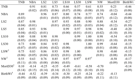
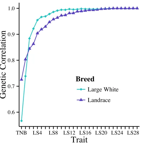
environment of the sow. Additive genetic variance was minimized at day 7 in Large White and day 14 in Landrace. Heritability estimates increased between TNB and LS30. Genetic correlations between TNB, NBA, and LS2-29 with LS30 plateaued within the first 10 days. A genetic correlation of 0.95 was reached at day 4 for Large White and day 8 for Landrace with LS30. Heritability estimates ranged from 0.07 to 0.13 for litter size traits and MortD30. Genetic correlations among LS30, LSW, and NW ranged from 0.97 to 1.00. Genetic

(2)

cross-fostering, and avoid back calculation associated with LS traits. Litter size at weaning would be optimal, but litter size at day 10 may be a compromise between genetic gain in litter size at weaning and minimizing the potentially negative effects of the nurse dam and additive genetics of the piglets as they are expected to increase throughout lactation. Final decisions need to be made on an individual breeding program basis.

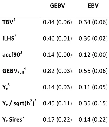
The objective of the second study was to determine the optimal validation method for comparing single-step GBLUP (GEBV) to pedigree (EBV) accuracy in litter size traits. Field data included six litter size traits: TNB, NBA, LS5, LS10, LSW, and NW. Simulated data was used to mimic the field data in order to select the method that was closest to the true accuracies (given the true breeding values were known). Six different methods were used to calculate the accuracy of both models. The methods used were: (1) traditional accuracy from the inverse of LHS (iLHS) using the standard error of prediction, (2) approximated

(3)

(4)

Alternative Litter Size Traits to Increase the Number of Weaned Pigs in Swine

by

Austin Michael Putz

A thesis submitted to the Graduate Faculty of North Carolina State University

in partial fulfillment of the requirements for the degree of

Master of Science

Animal Science

Raleigh, North Carolina 2015

APPROVED BY:

________________________________ ________________________________

Dr. Mark Knauer Dr. Christian Maltecca

Committee Chair

________________________________ ________________________________

(5)

DEDICATION

(6)

BIOGRAPHY

Austin Putz was born in Lacona, Iowa on December 4th, 1990, to Albert and Sherry Putz. He grew up with one older brother, Luke, a younger brother, Logan, and a younger sister, Brandi. He helped his dad run the farm growing up. They had cattle, pigs, and horses along with a few hundred acres of row crops. He graduated from Southeast Warren High School in May of 2009 and began his Bachelor’s of Science degree as an animal science student at Iowa State University. In May of 2013 he graduated with a B.S. in animal science.

As an undergraduate, he had several different jobs. First as a member of the Iowa State University Veterinary School barn crew. After that he moved on to work in a soils microbiology lab where he was exposed to new lab techniques. From there he moved to the department of animal science to work in two different molecular genetic labs. After

(7)

ACKNOWLEDGMENTS

I would like to first acknowledge Dr. Mark Knauer, my advisor, for taking me as a student and guiding me as a Master’s student. I appreciated his willingness to help and was always supportive. He allowed me freedom to take control of my own research and grow as a student and young scientist.

This project could not have been completed without the help and support of Smithfield Premium Genetics. Both of my summers were spent with them. All of their employees were extremely helpful throughout my entire project. It was a great environment to work while I was there.

I would like to thank Dr. Gene Eisen and Dr. O. W. Robison for coming to journal club over the last four semesters of my Master’s. During the semester it seemed like I didn’t have time, but looking back I realized I have learned a lot from our journal club sessions. It was great to sit down with other people and challenge each other’s thinking and points of view on topics not regularly discussed. It made me better as a researcher.

(8)

LIST OF TABLES

Table 1. Number of litters, sows, year-seasons, and farms for each breed ... 74 Table 2. Mean and SD for litter size traits, mortality, and birth weight in 8257 Large White and 6928 Landrace litters ... 75 Table 3. Additive genetic variance (!_!!_{), permanent environmental variance (}_!

!"! ), total variance (!!!),

and heritability (ℎ!_{) with standard errors (SE) for litter size traits, mortality, and birth weight in 8257}

(12)

LIST OF FIGURES

(13)

ABBREVIATIONS BLUP: best linear unbiased prediction

dEBV: deregressed estimated breeding value DGV: direct genomic breeding value

DYD: Daughter yield deviations EBV: Estimated breeding value

GEBV: genomic estimated breeding value LD: linkage disequilibrium

LE: linkage equilibrium

LS: litter size calculated as number of piglets assigned to the biological litter, usually followed by a number to indicate which day

LSY: litters per mated female per year MAS: marker assisted selection NBA: number born alive NW: number of weaned pigs

PSY: pigs weaned per mated female per year SSBR: single-step Bayesian regression models ssGBLUP: single-step genomic BLUP

(14)

LITERATURE REVIEW Introduction

One of the most economically important measures of sow production efficiency is the number of weaned pigs per mated female per year (PSY) (Amer et al., 2014). This can be broken down into two broad components, litters per mated female per year (LSY) and the number of weaned pigs per litter (NW).

Up until now, most breeding programs have focused on selection to increase litter size at birth, either total number born (TNB) or number born alive (NBA) with the

(15)

The first topic discussed will be a review on litter size at day 5. This is limited to two papers leaving a broader review to be completed on piglet survival, modeling, and associated variance components. Historically, piglet mortality has been modeled at the sow level, but has also been modeled at the piglet level to capture direct and maternal additive genetics along with the covariance between them.

The second topic discussed will be genomic selection. Genomic selection has become feasible for the industry due to advances in statistical methodology and affordable

genotyping. Capturing Mendelian sampling and correcting pedigree errors should increase accuracy of prediction, which should subsequently increase genetic progress.

Selecting for increased litter size at day 5, coupled with genomic selection will likely allow swine genetic companies to increase the rate of genetic improvement for litter size. This would result in improved commercial sow production given a sound genetic

implementation program. Litter size at day 5

It has been hypothesized that selection for litter size at birth has increased piglet mortality (Johnson et al., 1999; Lund et al., 2002), although the direct cause-effect

relationship has not been established. Litter size at day 5 is calculated by subtracting the sum of all piglet deaths up to day 5 from TNB. It is unique in that LS5 is calculated according to the biological dam, disregarding any cross-fostering that may have occurred. A justification for ignoring cross-fostering will be covered in the modeling section of this review.

(16)

calculated (i.e. deaths prior to this day/period are included). This will distinguish it from NW, which is based on the nurse dam and biological litter is ignored. Currently, only two papers exist on these new LS traits. First, Su et al. (2007) introduced the trait and investigated variance components associated with litter size and piglet survivability. Second, Nielsen et al. (2013) showed the response to selection for LS5 and the correlated responses in TNB and piglet mortality at day 5 (MortD5) over a six-year period. In 2004 the Danish breeding program replaced LS5 as the main maternal trait in place of TNB because of the unfavorable association that was observed between TNB and piglet survivability.

Su et al. (2007) was the first to introduce LS5. The objective of the authors was to investigate the genetic parameters among four litter size traits: TNB, NBA, LS5, and litter size at weaning of the biological dam (LSW) and three exclusive survival periods: at

(17)

modeling section of this review. From an implementation standpoint, the significance of LS5 is that it can be modeled at the sow level, not the piglet level.

Nielsen et al. (2013) were the second authors to investigate litter size at day 5. The main objective was to analyze the response to selection for LS5 after it became the main maternal trait in the Danish selection index starting in 2004 (Nielsen et al., 2013). Six years of data was analyzed from 2004 through 2009, with 7 different years of birth represented for genetic improvement. Phenotypic improvement was 1.4 and 2.1 piglets for LS5, 0.3 and 1.3 piglets for TNB, and 7.9 and 7.6% reduction in mortality at day 5 (MortD5) for Landrace and Yorkshire, respectively (Nielsen et al., 2013). More importantly, genetic improvement was 1.7 and 2.2 piglets for LS5, 1.3 and 1.9 piglets for TNB, and 4.7% and 5.9% for MortD5 for Landrace and Yorkshire, respectively (Nielsen et al., 2013). This clearly showed that

selection for LS5 successfully increased litter size at birth (TNB) and LS5 while decreasing MortD5 supporting the genetic correlations reported in Su et al. (2007). Although selection for LS5 would be successful in breeding programs, it is commonly argued that selection on component traits would be more effective (Knol et al. 2002a, Su et al. 2008). Since LS traits are a relatively new concept outside of Denmark, further research is needed to establish genetic parameters in differing populations. Prior to being implemented in breeding

programs, genetic correlations between LS traits and other traits of economic importance will need to be established.

Piglet Survival

(18)

environment play a role. Genetic ability includes both direct piglet and maternal components. Environmental factors are management including sow housing, husbandry, nutrition, cross-fostering practices, and processing (Lay 2002). Perhaps piglet survival has been viewed as a trait of the sow for simplicity. Modeling survival at the piglet level can complicate models and in the past was computationally too demanding (Knol et al., 2002a). In a later section the interaction between direct and maternal genetic components will be reviewed.

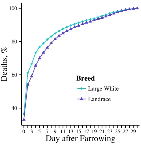
Piglet mortality can be split into two main phases, perinatal and postnatal causes. Perinatal mortality includes stillborns and mummified piglets, although the focus and emphasis is mainly put on stillborns because of the low percentage of mummified piglets. Often mummified piglets are ignored in the calculation of TNB. Postnatal mortality is any death occurring after the farrowing process. Low-vitality, overlying of the sow, disease, and starvation are generally accepted as the four main causes of postnatal mortality (English and Morrison, 1984). Piglet survival is most critical over the first few days of life (English and Morrison, 1984; Lay et al., 2002). In fact, over 50% of the deaths occur during the first 2 to 3 days of life (English and Morrison, 1984). This is because the main causes of death happen early on in lactation and piglets can control their environments more as they age (i.e. eating creep feed, drinking water, escaping from being crushed, etc.). Perhaps previous authors arbitrarily selected day 5 to signify early deaths (Arango et al., 2006; Su et al., 2007; Nielsen et al., 2013).

(19)

employee monitor the farrowing process and provide assistance if needed. This is especially important in the summer months when sows are more likely to become exhausted due to warm temperatures. Canario et al. (2006) reported that farrowing duration was the fourth largest cause of stillborns and may have increased in importance given the selection on litter size over the years. Other common management practices to reduce stillborns include inducing sows with lutalyse and administering oxytocin to improve uterine contractions.

Postnatal mortalities are harder to control from a management aspect. From 2008 to 2013, preweaning mortality increased 0.55% per year (Stalder, 2014). This demonstrates the unfavorable relationship with initial litter size that is commonly used as the main maternal trait. A common management practice to combat mortality that most production systems utilize is cross-fostering. The goal of cross-fostering is to give every piglet an equal opportunity to survive by moving some piglets to nurse dams or stated differently to accommodate the variation in rearing abilities of sows (Deen and Bilkei, 2004). Cross-fostering is usually performed within a few days of life. This should give every piglet an opportunity to feed while the sow is nursing (i.e. have enough functional teats to nurse all piglets). Utilization of heat lamps is a common way to reduce overlying of the sow. Placing a heat source away from the sow keeps piglets from laying close to the sow for warmth,

(20)

Modeling piglet survival

A common objection to LS traits is that they are modeled at the sow level. Main problems include, but are not limited to, ignoring additive genetics of the piglet (trait of the sow) and not accounting for nurse dam effects. Both the genotype of the sow and genotype of the piglet have an effect on piglet survival. Maternal influence decreases as the piglet ages and additive genetic variance of the piglet increases (Cassady et al., 2002; Su et al., 2008). Modeling piglet survival early in lactation should be less affected by not accounting for fetus/piglet genotype because that effect is very small (Su et al., 2008). It is harder to justify ignoring direct additive effects of the piglet when modeling piglet survival later in lactation. Modeled at the sow level, heritability of piglet survival dropped from 0.13 to 0.02 and 0.10 to 0.01 for survival at birth (SVB) to survival from day 6 to weaning (SVW) for Landrace and Yorkshire, respectively (Su et al., 2007). Modeled at the piglet level with essentially the same dataset, maternal heritability dropped from 0.06 to 0.03 and from 0.05 to 0.02 between SVB and SVW for Landrace and Yorkshire, respectively (Su et al., 2008). This provides some support for the use of LS5, because (1) direct genetics of the piglet early in lactation appears negligible and its removal simplifies the model (i.e. more parsimonious) and (2) over 50% of deaths prior to weaning occur during the first few days of life (English and Morrison, 1984), therefore capturing the majority of piglet mortality. Litter size at day 5 has the advantage of easily being implemented into current selection programs because most companies are still using litter size at birth modeled at the sow level.

(21)

weaned pigs. It is important to point out that there is an economic cost to piglets that are born and not weaned. Extra piglets take up resources in the uterus and nursing after parturition. Processing piglets that don’t make it to weaning is another economic cost to consider. Overall, if the goal is to directly select for piglet survival, it’s important to separate it into component traits.

The ability of a piglet to survive at farrowing is not the same trait as the genetic ability of a piglet surviving early and late in lactation. There are separate sets of fixed and random effects for the different survival traits (i.e. time periods). For instance, it doesn’t make sense to fit a nurse sow effect for piglet survival at farrowing; it has no biological meaning and would be completely confounded with maternal additive genetics. The

(22)

To the best of the author’s knowledge, only one attempt has been made to account for nurse sow effects in a model. The objective of Knol et al. (2002a) was to define the best model for birth weight and three piglet survival traits from combinations of direct, maternal, and nurse sow effects. Two lines were analyzed, a sire line and dam line. Results showed the best model for birth weight was a direct/maternal model (Knol et al., 2002a). Farrowing survival in the dam line was best fit by the direct model, while in the sire line both maternal and direct/maternal models fit the data equally well (Knol et al., 2002a). Preweaning survival was difficult to interpret because log-likelihood was used, which resulted in only nested models being comparable. It was concluded that the maternal/nurse sow model fit the data best (Knol et al., 2002a). Total survival, a combination of farrowing and pre-weaning survival, was also best fit with the maternal/nurse sow model (Knol et al., 2002a). One

should acknowledge that this research modeled piglet survival as a linear model, disregarding its threshold characteristic, which may have affected the results. Therefore, results may or may not be appropriate, but seem to make biological sense. Although models that fit nurse sow sometimes fit best, a main conclusion of the paper was that fitting nurse sow, as a whole, gave erratic results (Knol et al., 2002a). The same authors stated that relatively many piglets would need to be cross-fostered in order to accurately estimate both maternal and nurse sow effects (Knol et al., 2002a).

(23)

difficult to disentangle and therefore almost all studies have excluded the effect, even in preliminary analyses. Ideally cross-fostering would be designed from a statistical standpoint, which is perhaps unreasonable for farm staff to implement. Bouwman et al. (2010) tested social effects models and needed greater than 25% of the piglets cross-fostered to disentangle effects. In a production setting it may be best to leave as many piglets on the sow as possible without causing well-being issues. Workers may be biased toward one breed, cross-fostering more piglets onto one or the other because they are perceived to be superior in mothering ability and/or milking (Knol et al., 2002a). In many instances only one or two piglets are cross-fostered onto a nurse dam from a particular litter. Given a high turnover rate of females, the EBV for nurse dam would be poor.

One final concern is the ability of selection programs to accurately record piglet survival traits or even record them at all. Cross-fostering events are likely to be poorly recorded even in nucleus herds (personal communication). There is an economic cost and practical consideration to modeling piglet survival at the piglet level. At least some programs do not tag and record data for piglets that have died before processing. For example, 10 piglets are born in total, but only 7 are alive at processing. It makes little sense at a

production level to tag and record birth weights on the 3 that died so many systems do not simply because they were not using individual piglet information explicitly in their

(24)

a piglet existed, no birth weight would be available and the model could not be fit unless the data were imputed. This may not seem like a problem because a breeding program could decide to start recording all piglets, which would come at a slightly greater economic cost, but there may be a viable alternative (e.g. LS traits which only need the date of death on those piglets after processing, not before). Accuracy of recording quality of observations can also be questioned. In a production setting, qualification of piglet deaths as stillborn or an early preweaning mortality is perhaps questionable, especially if there are bonuses involved with meeting production levels. A reliable way of determining cause of death would be a thorough necropsy or floating a piece of the lung in water (Roehe et al., 2009). Piglet death classification with LS traits is irrelevant and selection has proven to be effective (Nielsen et al., 2013).

Variance components associated with piglet survival

Piglet survival is generally split into two broad categories or traits, perinatal survival and postnatal (preweaning) survival (Bidanel, 2011). Stillborns, and to a lesser extent mummified piglets, characterize perinatal survival, also referred to as farrowing survival. Many times it is calculated as the ratio of NBA to TNB if used as a trait of the sow. Stillborn piglets are a major cause of death across swine production systems. Postnatal mortality is defined as deaths of liveborn piglets. Some authors have chosen to split postnatal survival into two traits for a total of three piglet survival traits, including farrowing survival, as described above (Arango et al. 2006; Su et al., 2008).

(25)

2014). The same authors reported number born alive accounted for 27.1%; combined with piglet survival the total becomes 42% of the index (Amer et al., 2014). Although, one could argue that no economic weight should be placed on NBA or piglet survival given the classic selection index approach. In the classic aggregate genotype approach (Hazel, 1943), Pb = Gv. Vector v would include economic weights of “goal traits” while vector b would include weights for “selection criteria” traits. In practice, b would include NBA and piglet survival, while v should include NW or some variation of litter size at weaning. One argument could be that because NW is viewed an aggregate trait in itself and hard to manage because of cross-fostering, the G matrix would include poor estimates for the covariance between traits. Therefore it would be easier to consider NBA and piglet survival as goal traits themselves.

Perinatal Survival

Perinatal survival, also known as farrowing survival, includes stillborns and

(26)

Direct heritability averaged 0.06 and maternal heritability averaged 0.07 (Arango et al., 2006; Su et al., 2008; Roehe et al., 2010; Knol et al., 2002a; Ibáñez-Escriche et al., 2009).

Illustrating that slightly more influence comes from the dams’ genes as a mother. A fairly recent paper that focused on farrowing survival estimated direct and maternal heritability for three genetic lines of 0.02, 0.06, and 0.10, respectively for direct heritability, and 0.05, 0.13, and 0.06, respectively for maternal heritability (Ibáñez-Escriche et al., 2009).

Often journal articles on piglet survival do not attempt to address model selection, or if they do it’s not reported. Knol et al. (2002a) reported the maternal line fit farrowing survival best with only a direct effect, while the sire line fit best with a direct/maternal model. Nurse sow was of course not considered for farrowing survival because cross-fostering generally happens at a few days of age and the effect would have no biological meaning. It was not surprising that in both cases the maternal and direct/maternal models fit essentially the same based on the log likelihood (Knol et al., 2002a). Log likelihood makes model comparison easier because a p-value for differences in models can be obtained. The drawback is that no penalty is assigned for the number of parameters in the model. Selection criteria such as AIC or BIC would penalize more complex models like the direct/maternal model and favor a simpler model. When using log likelihood, if two models are not significantly different then one would choose the simpler model.

Postnatal Survival

(27)

postnatal survival averaged 0.05 over 12 estimates, slightly lower than farrowing survival (Bidanel, 2011). This is not surprising, as more environmental variability would be expected after farrowing such as disease and competition. However, there is little to no practical significance between 0.07 and 0.05 for estimates in The Genetics of the Pig (Bidanel, 2011). Direct heritability averaged 0.06 and maternal heritability averaged 0.07 in an independent review (Arango et al., 2006; Su et al., 2008, Roehe et al., 2010; Knol et al., 2002a; Ibáñez-Escriche et al., 2009). These estimates were identical to farrowing survival.

Direct and maternal additive genetic covariance

Many attempts have been made to characterize variance components associated with direct/maternal models. As previously described, rarely is nurse sow effect added to the model for piglet survival. Models that take into account the binary observation of piglet survival and the covariance structure from modeling direct and maternal additive genetic effects with the addition of the litter effect are commonly viewed as superior models. The downside is that these models add extra parameters for estimation, namely the covariance term between both effects. More parameters could lead to a problem of over-fitting, which in many cases can be more detrimental than having too simple of a model. This needs to be considered for genetic improvement because negative correlations between genetic parameters indicate that selection for one component (i.e. direct or maternal) may be

(28)

piglet level regardless of whether or not an antagonist relationship exists between the two. Yet an additive direct genetic effect for piglet survival in the paternal line(s) is sufficient. Perhaps these strategies would maximize survival in the offspring of the F1, the terminal crossbred animal. Attempts at quantifying the relative importance of piglet/embryo, maternal, and paternal effects for litter size have concluded that the largest part of the genetic variation is due to the genetics of the sow (Bidanel, 2011; Blasco, 1993).

(29)

Birth weight’s role in piglet survival

Litter size has increased dramatically over the last 20 years due to selection pressure owed to its large economic value (Amer et al., 2014). One major consequence of increasing litter size is the associated decrease in individual piglet birth weight, increase in variation for birth weight, and increase in preweaning mortality (Kerr and Cameron, 1995; Lund et al., 2002). Roehe (1999) estimated an additional piglet per litter reduced individual birth weight (IBW) by 44g. Biologically the association is easy to understand. As the number of piglets increases there are fewer resources per piglet for growth and development even though the total litter weight may still increase due to more piglets being born. A very close and well-known relationship exists between birth weight and piglet survival (English and Morrison, 1984). However, this relationship seems to be mainly phenotypic and to a lesser extent genetic (Knol et al., 2002b). Some authors in the past have suggested selection for birth weight will increase piglet survivability (Johnson et al., 1999; Roehe, 1999). Others suggest that within litter variability (or similar trait) may be more appropriate as discussed in a subsequent paragraph (Damgaard et al., 2003; Quesnel et al., 2008; Wolf et al., 2008).

(30)

the sow, litter birth weight heritability averaged 0.24 (Bidanel, 2011). These results show that direct selection on birth weight is possible, but less efficient than selecting for birth weight as a trait of the sow.

Selection for litter birth weight may be more effective because the heritability is between two and five times greater than the direct heritability (Bidanel, 2011). One problem with selection for birth weight is the existence of an unfavorable negative genetic correlation between direct and maternal components for birth weight in some studies (Roehe, 1999; Knol et al., 2002a; Su et al., 2008). The range is from -0.41 to 0.33 with a mean of -0.07 (Roehe, 1999; Knol et al., 2002a; Su et al., 2008; Grandinson et al., 2002). Given a large range, no inductive conclusion can be drawn from these studies. Perhaps genetic correlations between direct and maternal components for birth weight vary due to previous selection, data

collection procedures, and modeling. More research may need to be completed to thoroughly answer this question. Due to the possible unfavorable correlation between direct and

maternal components for birth weight, it may be necessary to model birth weight as a trait of the piglet and combine both direct and maternal components into the selection index like piglet survival.

As mentioned above, one alternative to average/individual birth weight is selection for within-litter variation in birth weight. The strong phenotypic relationship is well

(31)

2001). Wolf et al. (2008) proposed many different measures of variability for piglet birth weight including minimum, maximum, range, arithmetic mean, harmonic mean, variance, standard deviation, coefficient of variation (CV, %), and skewness. Results showed that average birth weight had a lower genetic correlation with losses from birth to weaning than SD and CV in birth weight (Wolf et al., 2008). Yet all three traits had similar genetic correlations with percentage of stillborn piglets (Wolf et al., 2008).

(32)

total number born or born alive. Arango et al. (2006) reported direct and maternal genetic correlations between birth weight and total mortality of -0.34 and -0.16, respectively. Stated more clearly, greater birth weight is associated with reduced mortality. The general

consensus is that almost every correlation is favorable between average birth weight or variation in birth weight and survival. However, Grandinson et al. (2002) did report an unfavorable genetic correlation between birth weight and total mortality of 0.19. In

circumstances where stillborns are the overwhelming majority of deaths, it seems more likely because of the unfavorable correlation between birth weight and stillborns. That is, selection for a birth weight trait will improve survival after farrowing, but it seems that it will be minimal and may come at a cost to increasing stillborns. This is because (1) the estimated heritability for birth weight is low (direct) to moderate (maternal) and (2) the genetic correlation between birth weight and survival appears low to moderate. A full economic evaluation of birth weight (both average and variation) would need to be completed taking into account the estimated variance components with all other economically important traits.

(33)

remains. It is this very competitive situation which prevails within litters for nutrition which puts the smaller piglet at such a distinct disadvantage relative to its larger littermate.” Knol et al. (2002b) is another popular review paper that stated, “These values cast some doubt on the approach of increasing survival through a genetic increase in birth weight.” Citing that the phenotypic correlation has been commonly misinterpreted as a genetic correlation in many instances (Knol et al., 2002b). The key is that this discussion pertains only to the relationship between piglet survival and birth weight. Some authors have suggested selection for

increased birth weight as a means to improve other traits such as carcass traits and growth (Fix et al., 2010a; Quiniou et al., 2002; personal communication). In summary, selection for individual birth weight and/or variation in birth weight (e.g. SD or CV) will not hurt piglet survivability, but may not increase survivability either.

(34)

for resources. As individual birth weights have decreased over the years, it has lead producers and researchers alike to believe that selection for birth weight will alleviate this problem.

Ethics

Societal pressures have begun to affect the swine industry. Recently, many top retailers of pork have decided they will start buying pork from gestation stall free systems (Merks et al., 2011). There is a concern for an updated breeding goal for companies. Pressure to remove gestation stalls has already affected retailers to put pressure on producers to move to stall free housing (Merks et al., 2011). Selection for piglet survival has an increasing economic and non-economic value due to societal pressures and may create marketing opportunities if a company can prove they have lower piglet mortality. Many ethical concerns have already been addressed in Europe (Merks et al., 2011). Perhaps it would be smart for US producers to stay ahead of society pressures and address them prior to becoming problematic.

Kanis et al. (2005) suggested a way of incorporating non-economic traits into the selection index. One problem with many of the traits suggested, such as feet and leg issues, is the lack of research on these traits. In fact, genetic correlations had to be fabricated in this study because no current estimates exist for them. Only conservative, biological estimates (educated guesses) could be made. This is far from ideal for breeding companies. Merks et al. (2011) suggested five broad categories that will need to be included in the future. New

(35)

begun to take effect in Europe and perhaps it’s only a matter of time before changes will be expected in the United States. It would be wise for companies to be proactive on many of these traits, especially traits with economic and non-economic value such as longevity and piglet vitality.

Molecular biology era

Since the days of Dr. Lush and Dr. Hazel, animal breeders have been focused on unmasking additive genetic values from phenotypes. They worked with the infinitesimal model introduced by Fisher (Fisher, 1918). The infinitesimal model is defined by having an effectively infinite number of loci causing very small effects. Henderson used this model to establish BLUP methodology (Henderson, 1976). Molecular biology as a field didn’t exist so animal breeding was limited to only the pedigree and phenotypes of individuals. In fact, at the time Animal Breeding Plans was first written it wasn’t certain how many chromosome pairs existed in all species (e.g. chicken, Lush, 1937). Despite not knowing about the ‘genetic architecture’ we speak of today, past geneticists made exceptional genetic improvement in many traits.

(36)

equilibrium, linkage disequilibrium (LD): loci that are in population-wide LD with the functional mutation, or direct markers (QTL): loci that code for the functional mutation (Andersson, 2002; Dekkers, 2004). Opportunities to discover markers caused a shift in funding from quantitative genetics to molecular genetics and was addressed by Misztal (2007) in an editorial of the Journal of Animal Breeding and Genetics, which has helped cause a shortage of animal breeders today.

Economically, the benefit of genotyping would be to reduce or even eliminate progeny testing of sires by utilizing molecular information, thus reducing cost and the generation interval. Dekkers and Hospital (2002) show a figure (3) in which offspring of a bull are genotyped and the one that received the favorable allele is then preselected for progeny testing. The cost of genotyping offspring would be only a fraction of the total cost of progeny testing all possible replacements (Schaeffer, 2006). However, its practical

application in commercial livestock improvement has been limited if not non-existent in many populations (Dekkers 2004; Dekkers 2012).

A review of MAS and its application in the commercial industry is provided by Dekkers (2004). In this review many problems with implementation are addressed. First, it’s difficult to apply an economic value to a single marker (Dekkers, 2004; personal

communication). It can be challenging to accurately apply economic weights to entire traits in different lines let alone one marker that may only exist in one line. Second, replication of QTL studies was rare, most likely due to insufficient LD between marker and QTL

(37)

be reviewed later. Experimental crosses were used extensively in QTL studies to create LD in populations (Andersson, 2001; Dekkers, 2004). Third, due to the polygenic nature of many economically important traits, many markers/QTL discovered only explained a limited proportion of the genetic variation (Dekkers, 2012). A challenge that is generally not discussed is the level of difficulty in applying MAS, which is less than straightforward (e.g. see Lande and Thompson, 1990). This concern has also been raised more recently with genomic selection (VanRaden, 2008). Many geneticists lacked experience and technical skill to implement MAS strategies because of the level of difficulty involved and logistical

problems of DNA collection and analysis (Dekkers, 2004). Overall, it seems MAS’s impact is minimal to this point. Industry leaders need the training and experience prior to

implementing these strategies because their decisions will affect their population long term. Prior to modern genomic selection, the idealized use of molecular information involved genotyping young animals with no phenotype and calculating the true breeding value. In an extreme case, velogenetics could be used to dramatically reduce generation interval. This procedure involves harvesting oocytes, fertilizing them, and genotyping prior to implantation into a donor (Georges and Massey, 1991). Traditionally in the key equation, there is a trade-off between accuracy and generation interval (Bourdon, 1997). In practice velogenetics is a long way off and unlikely, but genomics will eliminate this trade-off by increasing accuracy of prediction while simultaneously reducing generation intervals.

(38)

of single or multiple marker MAS (Meuwissen, 2001). Meuwissen et al. (2001) incorporated two fundamental approaches using genomics: genome wide association studies (GWAS) to locate and annotate candidate QTL nearby and utilizing dense markers to calculate breeding values. The idea was that by utilizing dense panels, all QTL would be in LD with at least one marker. Bayesian models were introduced to address the problem of having many marker effects to estimate with a limited amount of data (Meuwissen et al., 2001). Marker SNP effects became random and Gibbs sampling (along with Metropolis-Hasting) was

implemented to estimate all these effects simultaneously (Meuwissen et al., 2001). These SNP solutions could in turn be used for newly genotyped animals to predict their breeding values. This was a revolutionary idea in animal breeding, as molecular data had grown so big that quantitative geneticists were now able to use it on a large scale. Alternatively, these methods could be used to locate QTL throughout the genome by the utilization of LD between marker and QTL, known as GWAS (Meuwissen et al., 2001). These methods have been implemented to locate regions and hopefully one day will explain most of the variation in complex traits not only in animals, but also for human diseases to save lives. This however proved more difficult than first imagined (see Juran and Nazaridis, 2011, titled ‘Genomics in the Post-GWAS Era’) due to the small fraction of additive genetic variation that was

(39)

2012). The overall consensus is that after going away from the ‘black box’ approach, many involved with prediction of complex traits agree that GWAS is probably not enough or at least needs to be altered to include more than only additive effects (e.g. Daniel Gianola, personal communication).

In parallel with the discussion on challenges with MAS, genomics has had hurdles as well. The problems came on two levels, (1) the theory and research to test GS and (2)

implementation at the commercial level (e.g. genetic nucleus herds). Blasco and Toro (2014) reviewed the implementation of genomic selection thus far, which will continue to evolve. From a research perspective, statistical theory needed to be developed in order for it to be tested (e.g. Meuwissen et al., 2001; VanRaden, 2008; Hayes et al., 2009; Legarra et al., 2009). These papers will be described in more detail in the sections to follow. One of greatest initial challenges of GS, that was not present with MAS, was the estimation of a greater amount of effects than amount of data or lack of degrees of freedom, the ‘small n, large p’ problem (Gianola et al., 2009). Often, only hundreds or a few thousand phenotypic records exist to estimate between 10,000 to over 700,000 marker effects. This makes GS depend heavily on the number of observations and creates a massive over-fitting problem. Other questions arose for GS: how many SNPs are needed (i.e. marker density), computing costs, non-additive effects, across breed prediction, and the use of lower density panels in breeding programs for imputation (Blasco and Toro, 2014). From a commercial perspective,

economics and logistics appear to be the main barriers to implementation. Costs of genotyping with the 60K SNP panel at this time are >$100 per animal (personal

(40)

breakeven prices for GS. Yet the same authors did not account for the economic value of breeding companies utilizing genomic selection as a marketing tool (Blasco and Toro, 2014). Some companies may outsell competitors simply because their customers see GS as

innovative and on the cutting edge. Although there have been many challenges for genomic selection, it’s safe to say that genomic selection has arrived and is here to stay.

Methods of genomic selection

Two opposing views exist on how to best implement genomics into animal breeding. Solving for marker effects is the Bayesian approach while utilizing realized relationships is the opposing view. Meuwissen et al. (2001) introduced methods for solving for marker effects, as described above. Najati-Javaremi et al. (1997) introduced the total allelic relationship (TA), which would later be known as the genomic relationship matrix (G). It was not calculated in the same manner as models today, but the idea was identical. This matrix uses loci scattered across the genome to capture Mendelian sampling instead of using the traditional expected relationships given by the numerator relationship matrix (NRM, Henderson, 1976). Both methods of genomic selection will be described in more detail below.

At the most basic level, Bayesian GS involves estimating each SNP effect and then multiplying them by the genotypes and summing these effects for each animal. The basic Bayesian model is

!= !"+ !_!_!_!!_!"!_!+!! ,

(41)

and jth SNP, and ! is the vector of residuals. It’s important to note that not all SNP estimation methods are Bayesian, but they are the most common (see de los Campos et al., 2013).

Bayesian methods involve multi-step approaches. This is because the best response in training data to estimate SNP effects would be the true breeding value (TBV) (Meuwissen et al., 2001). This is usually not available so it typically requires (1) running a routine

(42)

response, not considering dEBV. Collectively, past studies indicate more research is needed with swine field data to decide which response is best. Perhaps the best methodology will depend on the situation (e.g. data and population structure).

Bayesian methods become complicated because of the many different models that have been proposed. Most share a common bond, but are all slightly different (see Figure 2 in de los Campos et al., 2013). BayesA and BayesB were the first Bayesian methods introduced to estimate marker effects (Meuwissen et al., 2001). Subsequently, Bayesian ridge regression (BRR), BayesC (Habier et al., 2011), and least absolute angle and selection operator

(LASSO) were introduced (Yi and Xu, 2008; Usai et al., 2009), which are all fairly common. Other less common methods have also been suggested, but beyond the scope of this review.

The Bayes alphabet comes with different prior distributional assumptions. There are four general types of prior distributions: Gaussian (normal), thick-tail (i.e. t-distribution), point of mass and slab, and the spike-slab distributions (de los Campos et al., 2013). BayesA assumes a t-distribution, which allows for a higher probability of moderate to large SNP effects. BayesB uses a mixture distribution with an assumed π value, which is the

(43)

(Yi and Xu, 2008). Because the π value may have influence over the analysis, some authors have chosen to estimate π instead of assigning it a prior (e.g. BayesCπ). A flat prior is usually only assigned to fixed effects, while marker specific variances are usually assigned a scaled inverted chi-square distribution which is determined by the degrees of freedom (!) and the scale parameter (S). Mostly because a scaled inverted chi-square can take a wide variety of shapes (i.e. flexible). For prediction purposes, most Bayesian methods perform very similarly and will be discussed in a following section (Habier et al., 2011; Heslot et al., 2012).

Genomic BLUP (GBLUP) is a method in which the numerator relationship matrix (A) is replaced by the realized or marker derived relationship matrix (G) (Habier et al., 2007; VanRaden, 2009; Hayes et al., 2009). VanRaden (2008) shows that a common calculation of G is

! =_! _!!_(!!!_!_!) ,

and Z is calculated by

! =!−! ,

where p is the allele frequency; matrix M is an !!!!! matrix with elements 0, 1, 2

(44)

M, which sets the mean SNP effect value to zero. GBLUP assumes SNP effects are normally distributed with a common variance (Mrode 2014).

In contrast to multi-step procedures, single-step GBLUP (ssGBLUP) combines pedigree, phenotypes, and genotypes into a single evaluation. Single-step GBLUP incorporates the realized relationship matrix (G) into a mixture relationship matrix (H), which is comprised of A partitioned into non-genotyped (A11) and genotyped (A22) and G

(Legarra et al., 2009; Christensen and Lund, 2010). Originally the first derivation of the single-step approach was incorrect because the authors didn’t consider the joint distribution of both genotyped and non-genotyped individuals (Misztal et al., 2009). The correct

computation of H is fairly complex,

! =! !!!+ !!! !!!!"!!!"(!!!)!! −(!!!)!!!!"! −!!!"₍_!!!₎!! _! ,

however, the computation of it’s inverse has a very simple form (Aguilar et al., 2010),

!!! ₌_!!!₊ 0 0

0 !!!₋_!

!! !! ,

the important thing to realize about H is that it not only alters relationships between

(45)

albeit only slightly. The two main advantages of ssGBLUP are that it’s extremely simple to integrate into existing software because A-1_{is simply replaced by}_H-1_{and it directly}

computes GEBVs, eliminating multiple-steps in genomic evaluations.

Although GBLUP and/or ssGBLUP are viewed as very simple, calculating G has been a topic of debate (VanRaden 2008). Allele frequencies of the base population are needed to create G. In reality these don’t exist (currently) and are usually replaced by observed allele frequencies of the sample. This was found to have little influence in a

simulation study (VanRaden, 2008). Standardization of G has also been debated. Forni et al. (2011) suggested that the average diagonals of G should equal the average diagonals of A22.

Others have suggested that a small value should be added to all elements of G (Chen et al., 2011; Vitezica et al., 2011). Combining these ideas yielded setting the average diagonals of G equal to the average diagonals of A22 and the average off-diagonals of G to the average

off-diagonals of A22 and solving for ! and ! (Guo et al., 2015). Not only can G be weighted

with A22 to yield G*, but G*-1 and A-1 can be weighted inside H as well. This is best

illustrated in an equation taken from Lourenco et al. (2014)

!!!₌ _!!!₊ 0 0

0 ! !!+!!!_!! !!₋_!_!!

!!

!! ,

where H, G, and A were defined earlier and !, !, !, ! are weighting parameters for G*-1, !_!!!!_,_A_{, and}_G_{, respectively. One final problem is that}_G_{may not be semi-positive definite.}

(46)

Single-step GBLUP is very appealing because of its simplicity in being able to combine genotyped and non-genotyped animals easily into one model. Field populations are likely to never include genotypes for every individual in the database, although genotyping costs will continue going down. Traditional multi-step procedures for genomic selection cannot incorporate non-genotyped animals like ssGBLUP, although they do contribute to the pseudo phenotypes. In response, Fernando et al. (2014) derived a novel method for Bayesian models to incorporate non-genotyped animals. One problem with ssGBLUP is the need to compute the inverse of the very dense G matrix. Currently, there seems to be no simple solution for the direct calculation of the inverse of G, such as the one for A inverse

(Henderson, 1976). One method using a similar recursion technique has been proposed, but has not been tested extensively (Misztal et al., 2014). Single-step Bayesian regression models (SSBR) will be able to handle a larger number of individuals because it avoids the dense matrix inversion of ssGLUP (Fernando et al., 2014). The cost scales linearly with the number of non-genotyped and genotyped animals (Garrick et al., 2014). These models have recently been developed so testing and comparison of these models with traditional Bayesian multi-step, GBLUP, and ssGLUP are likely to follow. The downside is that implementation into existing software may be slow or limited because of the structure of the mixed model equations (e.g. alteration of the fixed-effects design matrix X) as mentioned in a review by Garrick et al. (2014).

Accuracy of prediction

(47)

VanRaden, 2008). In simulation studies true breeding value (TBV) is known. One can obtain a measure of accuracy simply by calculating the correlation between TBV and the estimated breeding value (with or without genomics). In traditional evaluations, the inverse of the diagonals in the left hand side (LHS) were used from the mixed model equations (Mrode 2014). Many methods that estimate marker effects never set up the mixed model equations (or can’t be inverted) and therefore can’t be used to get the theoretical accuracy. Hence, perhaps a validated accuracy is better because animal breeders need the ability to predict breeding values into the future (i.e. young sires). Using LHS inverse elements in GBLUP approaches where the MME are set up, it becomes dependent on allele coding and weighting of the matrices (A and G), although it has been done (e.g. Forni et al., 2011). Genomic selection with field data requires alternate methods of achieving a measure of accuracy because TBV is an unknown value. Many times cross-validation or forward validation is applied. The first by splitting the dataset randomly into several groups and the latter by cutting at one specific time and predicting the young animals EBV with no phenotype (masked). The two resulting datasets are referred to as training and validation datasets. Alternatively, one can split based on family structure or subpopulation structure in plants to cross-validate accuracy (Saatchi et al., 2011; Usai et al., 2009; Heslot et al., 2012). The validation response is a highly accurate EBV, daughter yield deviation (DYD, for sires), corrected phenotypes, or dEBV from the traditional evaluation.

(48)

accuracy may be challenging because there are many methods that can vary slightly and many ways to calculate accuracy. For this reason, most results will not present values, only a better/worse conclusion.

Meuwissen et al. (2001) used four models for prediction: least-square estimation (LS), best linear unbiased prediction (BLUP), BayesA, and BayesB. The same authors used forward validation by calculating prediction equations in a training dataset and then using them in the next two generations with no phenotypes. Overall, BayesB outperformed other models for location of QTL and accuracy of prediction, with BayesA being slightly lower (Meuwissen et al., 2001). Conclusions were (1) it is possible to accurately predict breeding values using a dense marker map, (2) prior distribution assumptions had little effect on prediction of breeding values, and (3) selection on predicted breeding values predicted could substantially increase the rate of genetic gain by increasing accuracy and reducing generation intervals (Meuwissen et al., 2001). This paper also showed how accuracy is dependent upon the size of the reference population, is influenced by marker density, and how accuracy declines over generations due to the breakdown of LD. This was a landmark paper because it was the first time that breeding values had been predicted solely from marker data in young individuals.

(49)

Hospital 2002). A weakness of simulation studies is that the model used to create the simulation is also used to analyze the data (i.e. additive model, Blasco and Toro, 2014). Therefore they should be used more for methodology and care should be taken in interpreting the results.

Christensen et al. (2012) compared pedigree predictions to GBLUP, regular ssGBLUP, and an adjusted ssGBLUP. All three GBLUP methods outperformed pedigree predictions and yielded similar accuracies among genomic methods for feed conversion ratio and ADG in univariate and bivariate models (Christensen et al., 2012). An advantage of ssGBLUP over Bayesian methods is the direct integration into multi-trait models, which can further increase prediction accuracy (Legarra et al., 2014). Single-step GBLUP could

therefore offer additional accuracy. Gu et al. (2015) confirmed the advantage of using the G matrix for litter size by comparing pedigree, GBLUP, and ssGBLUP. Averaged across traits (TNB, LS5, and MortD5), ssGBLUP roughly doubled the pedigree accuracy (0.091 versus 0.213, Gu et al., 2015). Tusell et al. (2013) was the first to comprehensively review marker estimation methods for prediction of litter size. The authors compared models that were linear and non-linear such as Bayesian Lasso, ridge regression, reproducing kernel Hilbert spaces (RKHS), GBLUP, and neural networks. The conclusion was that genomic methods substantially improved prediction over the pedigree, but all performed roughly the same (Tusell et al., 2013). The authors suggested that perhaps Bayesian neural networks provide an advantage in F1 prediction as they analyzed the crossbred performance with genotypes

(50)

effects, which becomes more important in crossbreds. In dairy sheep, it was concluded that recorded phenotypes in ssGBLUP resulted in a 9% increase in accuracy and lower bias averaged over seven traits when compared to using pseudo phenotypes for ssGBLUP (Baloche et al., 2014).

Comparison of the marker estimation methods to ssGBLUP for genomic prediction

For practical purposes, breeding programs need to know which methodologies are superior and which are easiest to integrate into their current selection program. Relatively few papers exist comparing marker estimation methods to ssGBLUP because many authors favor one over the other (see Forni et al., 2011 and Habier et al., 2011). Legarra et al. (2014) recently reviewed ssGBLUP and only reported four estimates that compared ssGBLUP and multi-step approaches. GBLUP has been compared to marker estimation methods many times, however studies usually involve using a pseudo phenotype and are not readily applicable to livestock populations because many non-genotyped individuals have phenotypes. Utilizing ssGBLUP easily integrates phenotypes, pedigree, and genomic information in a simple way; perhaps it makes basic GBLUP irrelevant because it’s more difficult to implement and less accurate than ssGBLUP (Guo et al. 2015; Gao et al., 2012). However, because more estimates exist between marker methods and GBLUP they will be used as well.

(51)

2010). It should be clarified that just because very large QTL(s) have been identified (e.g. DGAT1 for fat percent in dairy), that doesn’t mean there are few QTL. Therefore, the study by Daetwyler et al. (2010) wasn’t exactly representative of the genetic architecture that may exist for some traits. The same authors stated the remaining additive variance could follow the infinitesimal model with hundreds or thousands of QTL. Yet no results were shown. It was concluded that the advantage of BayesB or GBLUP depends on three things: the population genome structure (Ne), genetic architecture (h2_{and NQTL), and the size of the} training set (Daetwyler et al., 2010). These are the same three factors that affect overall accuracy of genomic selection. Single-step GBLUP assumes the infinitesimal model

(approximately), therefore it doesn’t account for traits with very large QTL effectively. This is because there is only one variance parameter and therefore ssGBLUP shrinks all marker effects the same. To the best of the authors’ knowledge, no swine paper has been published comparing ssGBLUP to marker estimation methods and only one that has compared GBLUP to marker estimation methods (Ostersen et al., 2011). Therefore extrapolations will need to be taken from other species.

(52)

accuracies of genomic predictions. Aguilar et al. (2010) compared an unspecified multi-step procedure to many different versions of ssGBLUP in the computation of G and H. The multi-step procedure gave a validated accuracy of 0.40, while the average ssGBLUP was 0.39 (Aguilar et al., 2010).

In light of these results, it’s unsurprising that some swine breeding companies have already implemented GS in the form of ssGBLUP as stated above (personal communication). This mostly likely has very little to do with the slight advantage of ssGBLUP in some cases, but more to do with the ease of implementation (personal communication). Breeding

(53)

LITERATURE CITED

Aguilar, I., I. Misztal, D. L. Johnson, A. Legarra, S. Tsuruta, and T. J. Lawlor. 2010. Hot topic: A unified approach to utilize phenotypic, full pedigree, and genomic

information for genetic evaluation of Holstein final score. J. Dairy. Sci. 93:743-752. Amer, P. R., C. I. Ludemann, S. Hermesch. 2014. Economic weights for maternal traits of

sows, including sow longevity. J. Anim. Sci. 92:5345-5357.

Andersson, L. 2001. Genetic dissection of phenotypic diversity in farm animals. Nat. Rev. Genet. 2:130-138.

Arango, J., I. Misztal, S. Tsuruta, M. Culbertson, J. W. Holl, and W. Herring. 2006. Genetic study of individual preweaning mortality and birth weight in Large White piglets using threshold-linear models. Livest. Sci. 101:208-218.

Baloche, G., A. Legarra, G. Salle, H. Larroque, J. M. Astruc, C. Robert-Granie, and F. Barillet. 2014. Assessment of accuracy of genomic prediction for French Lacaune dairy sheep. J. Dairy Sci. 97:1107-1116.

Bidanel, J. P. 2011. Biology and genetics of reproduction. In: M. F. Rothschild and A. Rubinsky, editors, The genetics of the pig. 2nd ed. C.A.B. International, Oxfordshire, UK. p. 218-241.

Blasco, A. 1993. The genetics of prenatal survival of pigs and rabbits: a review. Livest. Prod. Sci. 37:1-21.

(54)

Bourdon, R. M. 1997. Understanding Animal Breeding. Prentice Hall, Upper Saddle River, NJ. 2nd edition.

Bouwman, A. C., R. Bergsma, N. Duijvesteign, and P. Bijma. 2010. Maternal and social genetic effects on average daily gain of piglets from birth until weaning. J. Anim. Sci. 88:2883-2892.

Canario, L., E. Cantoni, E. Le Bihan, J. C. Caritez, Y. Billon, J. P. Bidanel, and J. L. Foulley. 2006. Between-breed variability of stillbirth and its relationship with sow and piglet characteristics. J. Anim. Sci. 84:3185-3196.

Cassady, J. P., L. D. Young, and K. A. Leymaster. 2002. Heterosis and recombination effects on piglet growth and carcass traits. J. Anim. Sci. 80:2286-2302.

Chen, C. Y., I. Misztal, I. Aguilar, A. Legarra, and W. M. Muir. 2011. Effect of different genomic relationship matrices on accuracy and scale. J. Anim. Sci. 89:2673-2679. Christensen, O. F. and M. S. Lund 2010. Genomic prediction when some animals are not

genotyped. Gen. Sel. Evol. 42:2.

Christensen, O. F. P. Madsen, B. Nielsen, T. Ostersen, and G. Su. 2012. Single-step methods for genomic evaluation in pigs. Animal. 6:10:1565-1571.

Daetwyler, H. D., R. Pong-Wong, B. Villanueva, and J. A. Woolliams. 2010. The impact of genetic architecture on genome-wide evaluation methods. Genetics. 185:1021-1031. Damgaard, L. H., L. Rydhmer, P. Lovendahl, and K. Grandinson. 2003. Genetic parameters

(55)

de los Campos, G., J. M. Hickey, R. Pong-Wong, H. D. Daetwyler, and M. P. L. Calus. 2013. Whole-genome regression and prediction methods applied to plant and animal

breeding. Genetics. 193:327-345.

Deen, M. G. H. and G. Bilkei. 2004. Cross fostering of low-birthweight piglets. Liv. Prod. Sci. 90:279-284.

Dekkers, J. C. M. and F. Hospital. 2002. The use of molecular genetics in the improvement of agricultural populations. Nat. Rev. Genet. 3:22-32.

Dekkers, J. C. M. 2004. Commercial application of marker- and gene-assisted selection in livestock: Strategies and lessons. J. Anim. Sci. 82:E313-E328.

Dekkers, J. C. M. 2012. Application of genomic tools to animal breeding. Current Genomics. 13:207-212.

English, P. R., and V. Morrison. 1984. Causes and prevention of piglet mortality. Pig News Info. 5:369-376.

Fernando, R. L., and M. Grossman. 1989. Marker assisted selection using best linear unbiased prediction. Genet. Sel. Evol. 21:467-477.

Fisher, R. A. 1918. The correlation between relatives on the supposition of Mendelian inheritance. Trans. Roy. Soc. Edinburgh 52:399-433.

(56)

Fix. J. S., J. P. Cassady, J. W. Holl, W. O. Herring, M. S. Culbertson, and M. T. See. 2010b. Effect of piglet birth weight on survival and quality of commercial market swine. Livest. Sci. 132:98-106.

Gao, H., O. F. Christensen, P. Madsen, U. S. Nielsen, Y. Zhang, M. S. Lund, and G. Su. 2012. Comparison on genomic predictions using three GBLUP methods and two single-step blending methods in the Nordic Holstein population. Gen. Sel. Evol. 44:8. Garrick, D. J., J. F. Taylor, and R. L. Fernando. 2009. Deregressing estimated breeding

values and weighting information for genomic regression analyses. Gen. Sel. Evol. 41:55.

Garrick. D. J., J. C. M. Dekkers, and R. L. Fernando. 2014. The evolution of methodologies for genomic prediction. Livest. Sci. 166:10-18.

Georges, M., J. M. Massey 1991. Velogenetics, or the synergistic use of marker assisted selection and germ-line manipulation. Theriogenology. 35:220-227.

Gianola, D., G. de los Campos, W. G. Hill, E. Manfredi, and R. Fernando. 2009. Additive genetic variability and the Bayesian alphabet. Genetics. 183:347-363.

Grandinson, K., M. S. Lund, L. Rydhmer, and E. Strandberg. 2002. Genetic parameters for the piglet mortality traits crushing, stillbirth, and total mortality, and their relation to birth weight. Acta Agric. Scand., Sect. A. Anim. Sci. 52:167-173.

(57)

Guo, G., M. S. Lund, Y. Zhang, and G. Su. 2010. Comparison between genomic predictions using daughter yield deviation and conventional estimated breeding value as response variables. J. Anim. Breed. Genet. 127:423-432.

Guo, X., O. F. Christensen, T. Ostersen, Y. Wang, M. S. Lund, and G. Su. 2015. Improving genetic evaluation of litter size and piglet mortality for both genotyped and

nongenotyped individuals using a single-step method. J. Anim. Sci. 93. 503-512. Habier, D., R. L. Fernando, and J. C. M. Dekkers. 2007. The impact of genetic relationship

information on genome-assisted breeding values. Genetics. 177:2389:2397.

Habier, D., R. L. Fernando, and J. C. M. Dekkers. 2011. Extension of the Bayesian alphabet for genomic selection. BMC Bioinformatics. 12:186.

Hayes, B. J., P. M. Visscher, and M. E. Goddard. 2009. Increased accuracy of artificial selection by using the realised relationship matrix. Genet. Res. Camb. 91:47-60. Hazel, L. N. 1943. The genetic basis for constructing selection indexes. Genetics. 28:476-

490.

Henderson, C. R. 1976. A simple method for computing the inverse of the numerator relationship matrix used in prediction of breeding values. Biometrics. 32:69-83. Hermesch, S. B., G. Luxford, and P. R. Amer. 2001. Genetic parameters for piglet mortality,

within-litter variatoin of birth weight, litter size and litter birth weight. In: Proc. Assoc. Adv. Anim. Breed. Genet., Queenstown, NZ. 14:211-214.

(58)

Hogberg, A. and L. Rydhmer. 2000. A genetic study of piglet growth and survival. Acta. Agric. Scand. Sect. A Anim. Sci. 50:300-303.

Johnson, R. K., M. K. Nielsen, and D. S. Casey. 1999. Responses in ovulation rate, embryonal survival, and litter traits in swine to 14 generations of selection to increased litter size. J. Anim. Sci. 77:541-557.

Juran, B. D. and K. N. Lazaridis. 2011. Genomics in the post-GWAS era. Seminars in Liver Disease. 31:215-222.

Kerr, J. C. and N. D. Cameron. 1995. Reproductive performance of pigs selected for components of efficient lean growth. Anim. Sci. 60:281-290.

Knol, E.F. 2001. Genetic aspects of piglet survival. Wageningen University, Wageningen, The Netherlands, Ph.D. dissertation.

Knol, E. F., B. J. Ducro, J. A. M. van Arendonk, and T. van der Lende. 2002a. Direct, maternal and nurse sow genetic effects on farrowing-, pre-weaning- and total piglet survival. Livest. Prod. Sci. 73:153-164.

Knol, E. F., J. I. Leenhouwers, and T. van der Lende. 2002b. Genetic aspects of piglet survival. Livest. Prod. Sci. 78:47-55.

Lande, R. and R. Thompson. 1990. Efficiency of marker-assisted selection in the improvement of quantitative traits. Genetics. 124:743-756.

Lay, D. C., R. L. Matteri, J. A. Carroll, T. J. Fangman, and T. J. Safranski. 2002. Preweaning survival in swine. J. Anim. Sci. 80:E74-E86.

(59)

Legarra, A., O. F. Christensen, I. Aguilar, and I. Misztal. 2014. Single step, a general approach for genomic selection. Liv. Sci. 166:54-65.

Lund, M. S., M. Puonti, L. Rydhmer, and J. Jensen. 2002. Relationship between litter size and perinatal and pre-weaning survival in pigs. Anim. Sci. 74:217-222.

Lush, J. L. 1937. Animal Breeding Plans. Collegiate Press Inc, Ames, IA.

McKay, R. M. 1993. Preweaning losses of piglets as a result of index selection for reduced backfat thickness and increased growth rate. Can. J. Anim. Sci. 73:437-442.

Meiwissen, T. H. E., B. J. Hayes, and M. E. Goddard. 2001. Prediction of total genetic value using genome-wide dense marker maps. Genetics. 157:1819-1829.

Meiwissen, T. H. E. 2007. Genomic selection: marker-assisted selection on a genome wide scale. J. Anim. Breed. Genet. 124:321-322.

Merks, J. W. M., P. K. Mathur, and E. F. Knol. 2011. New phenotypes for new breeding goals in pigs. Animal. 6:4.

Milligan, B. N., D. Fraser, and D. L. Kramer. 2002. Within-litter birth weight variation in the domestic pig and its relation to pre-weaning survival, weight gain, and variation in weaning weights. Livest. Prod. Sci. 76:181-191.

Misztal, I. 2007. Shortage of quantitative geneticists in animal breeding. J. Anim. Breed. Genet. 124:255-256.

(60)

Misztal, I., A. Legarra, and I. Aguilar. 2014. Using recursion to compute the inverse of the genomic relationship matrix. J. Dairy Sci. 97:3943-3952.

Mrode, R. A. 2014. Linear Models for the Prediction of Animal Breeding Values. 3rd Edition. CABI Oxfordshire, UK.

Nejati-Javaremi, A., C. Smith, and J. P. Gibson. 1997. Effect of total allelic relationship on accuracy of evaluation and response to selection. J. Anim. Sci. 75:1738-1745. Nielsen, B., G. Su, M. S. Lund, and P. Madsen. 2013. Selection for increased number of

piglets at d 5 after farrowing has increased litter size and reduced piglet mortality. J. Anim. Sci. 91:2575-2582.

Ostersen, T., O. F. Christensen, M. Henryon, B. Nielsen, G. Su, and P. Madsen. 2011. Deregressed EBV as the response variable yield more reliable genomic predictions than traditional EBV in pure-bred pigs. Gen. Sel. Evol. 43:38.

Quesnel, H., L. Brossard, A. Valancogne, and N. Quiniou. 2008. Influence of some sow characterisitcs on within-litter variation of piglet birth weight. Animal. 2:12:1842-1849.

Quiniou, N., J. Dagorn, and D. Gaudre. 2002. Variation of piglets’ birth weight and consequences on subsequent performance. Livest. Prod. Sci. 78:63-70.

Roehe, R. 1999. Genetic determination of individual birth weight and its association with sow productivity traits using Bayesian analyses. J. Anim. Sci. 77:330-343.

(61)

and individual birth weight on first generation data of a selection experiment for piglet survival under outdoor conditions. Livest. Sci. 121:173-181.

Roehe. R., N. P. Shrestha, W. Mekkawy, P. W. Knap, K. M. Smurthwaite, S. Jarvis, A. B. Lawrence, and S. A. Edwards. 2010. Genetic parameters of piglet survival and birth weight from a two