Abstract—Detection of outlying ratings of samples is a primary step in statistical analysis and classification. A novel rule-based method is presented for automatically detecting and removing outlying ratings in order to improve the quality of sample classification and to increase the degree of agreement between raters. The effectiveness of our method in improving the degree of agreement, assessed using a modified Fleiss' kappa, is demonstrated through a practical example. Our method is conceptually transparent, computationally simple and easy to apply in practice. It is expected to be a useful tool in many real world applications.
Index Terms—Outlying rating detection (ORD), rating frequency distributions, reliability of agreement
I. INTRODUCTION
Sample rating is an important tool and is widely used in industry, psychology, politics and commercial market research, it is also widely used in medical statistics and in food, social and many areas of science. In industry research,many organisations (i.e., banks, telecommunication companies, insurance companies, etc.) track and analyse consumer sentiment for service quality or customer satisfaction [1]. In market research, customers may be asked about their attitudes, perceptions or evaluations of products (or, foods, brands, etc.); managers maybe asked to rate their company's performance (type of strategic focus, degree of marketingexcellence, etc.) [1]. Studies [5], [6] show that 20% of data produced by medical researchis in ordered categories; quality assurance in hospitals may result in an increase in the useof methods which produce data in ordered categories [2]. Also, analysis of subjective measurements arises in many research areas, in particular, those concerning sensory testing orattitude scaling [8].
Automatic Outlying Rating Detection (ORD) is an important issue for many real world applications involving sample (data) gathering, analysis, ratings and classification (with ordered categories). A sentiment analysis system and its classifier, for instance, generally rely on the quality of classification of samples in order to accurately predict sentiment orientation of texts or sentences. While many samples, such as reviews rated by web users, are inherently likely to show differences in opinions, a robust and reliable ORD is a prerequisite for effective prediction.
An important area closely related to the current study is outlier detection. The definition of an outlier depends on underlying assumptionsregarding the detection method and data structure [2]. Generally, an outlier may be defined as a data point that “appears to deviate markedly from other
Manuscript received July 30, 2012; revised September 2, 2012. The authors are with School of Computing and Engineering, University of Huddersfield, HD1 3DH, UK (e-mail: [email protected], [email protected])
members of the sample in which it occurs” [1], [6]; or, “lies outside some overall pattern of distribution” [9]. A typical outlier detection technique is to characterise what ‘normal’ data points look like, and then to single out those data points that deviate from these normal properties [15]. There exist many outlier detection methods. A good review of outlier detection methods can be found in, for instance [2], [7].
An outlying rating of a given sample, as referred to in this study, is a rating appearing todeviate significantly from the majority of ratings of the sample. Outlying ratings may arisefrom experiment design errors and/or human-related errors, unrepresentative assessmentsor measurements, and so on. Outlying ratings often cause confusion for classification anddecrease prediction accuracy. However, the practical and important issue of automatic ORDremains to be developed.
The current study explores a rule-based method for automatic ORD of individual samples.The aim of this pioneering study is to improve the quality of sample classification and toincrease the degree of agreement between raters regarding the whole sample set. There are severalstatistics, for instance, [3], [4], [7], that measure the degree (reliability) of agreement achievedbetween more than two different raters rating the same samples. Fleiss' kappa measure [3]is simple and commonly used and, thus, it is used in our study. Note that thekappameasure assumes that the number of raters per sample must be fixed, although differentsamples may be rated by different raters. Therefore, in the current study, we also modify the kappa measure toallow the number of raters to vary from sample to sample. To the best knowledge of theauthors, our method is developed for the first time and is expected to be a useful toolfor state-of-the-art machine learning methods.
This paper is organized as follows. After giving a notation through aworking example in Section II, we introduce a series of basic concepts in Section III. We present a rule-based method for detecting and removing outlying ratings in Section IV and then discuss the extension of our method in Section V. We investigate to what extent our method contributes toincreasing the degree of agreement between raters through a practical example in Section VI, and draw conclusions in Section VII.
II. NOTATION
Sample rating, as used in this paper, refers to the process of assigning to each sample somevalue selected from a list predefined from a given ordered series. The values may be thoughtof as strength, extent, level, closeness, and so on, depending on the application. In effect, sample rating is equivalent to ‘sample classification’ if each value in the series correspondsto a category. Accordingly, the categories should be clearly defined, ordered and mutuallyexclusive. In
A Rule-Based Method for Outlying Rating Detection
what follows, we will regard the phrases ‘sample rating’ and ‘sample classification’ as interchangeable.
To begin with, let us give the representation of sample ratings.Suppose we have nsamples, denoted by
, , … , , of analysis and that we have Nvalues, denoted
by , , … , , predefined from a given
orderedseries. Suppose we have a classification, denoted by
S , , … , , over , which is a list of ordered
categories. We assume that each Scorrespondsto , where 1,2, … , . Suppose there are a total of mraters, and each of them is asked to assign a valueto some samples. We call the assignment a rating. In the end, from mraters, we obtain arating frequency for each of N values. Then we may represent the ratings of all the samples using an n-by-N table: the samples and values (categories) arepresented in rows and columns, respectively. The table contains
cells, and the , thcell contains the rating frequency, denoted by ri, j, which is the number of raters who assigned
sample siwith value vj(or, who classified the ith sample si
into the jth category Sj). Clearly, table ignores information
about raters themselves.
A typical application of ORD is in the area of sentiment analysis [14] and this is where our examples areset. The following working example, Example 2.1 will be usedthroughout this paper.
Example 2.1.Suppose we have a set of n = 6 samples, and
that there are m = 30 raters who were randomly selected and required to classify each sample into N=11 categories. Table I below depicts the statistics (see details in Section VI.B).
TABLEI:RATING FREQUENCIES FOR AN ORDERED CLASSIFICATION
-5 -4 -3 -2 -1 0 1 2 3 4 5
S \ S S1 S2 S3 S4 S5 S6 S7 S8 S9 S10 S11
s1 1 2 1 2 3 1 6 9 5
s2 1 7 8 4 2 1 2 1 2 1 1
s3 1 2 1 2 1 3 10 6 4
s4 3 7 4 7 3 2 1 2 1
s5 1 1 3 6 10 4 3 1 1
s6 1 1 1 5 6 7 9
Thus, from Table I, we haveS , , … , ,
5, … , 1,0,1, … ,5 andS , … , , , , … , , and
the (3, 9)th cell contains the rating frequency, r3,9 = 10,
which indicates that 10 ratersassigned sample s3 with value
v9 = 3 (or, classified sample s3 into category S9). ◊
III. CONCEPTS
This section introduces a series of basic concepts,which are used for characterising the ratingfrequency distributions of the individual samples. With these concepts, establishing the rules used in our method becomes straightforward.
Generally, there are three variables related to a given sample :
1) the number of raters who rated sample si:
,
2) an1-by-N matrix of rating frequencies of si over S:
, , , , … , , , … , , , ,
3) the distribution of rating frequencies of si over S:
, , , , … , , , … , , , ,
For a given with the rating frequency matrix ri (or,
ratings ri, in short),consider two arbitrary , S(where ). In current study, the order of the categories in Sis necessary. Thus we say if . We can define neighbour distance by the following statements. • The distance between and is defined by
, , | |
• The neighbour distance is a predefined parameter (a non-negative integer); we say is a neighbour of if
,
A dominant category, which is an important concept of ORD, in this study is the mode of the ratings ri.That is, a
category Sis said to be a dominant category of sample
, denoted by S*, if the corresponding rating frequency, denoted by , , satisfies
, , , ; 1
Obviously, each si has at least one dominant category.
The main category, which is another important concept of ORD, is the set of neighbouringcategories of the dominant category. That is, supposeS* = Sj is the dominant category of
, the main category of S*, denoted by [S*], is defined by
; , , 1
where is neighbour distance.
The left and right main categories of S* are definedrespectively by
; and 1
; and j
With the above concepts, in what follows, we will denote:
, ,
, ,
IV. OUTLYING RATING DETECTION (ORD)
This section presents our methodby establishing a series of rules for automatic ORD. The basic idea behind our method is simple: the dominant category is astarting point of ORD, which is taken as the highest frequency of ratings for eachgiven sample. There may be alternative ways to define the dominant category, depending onthe application. We use the mode for two reasons: (i) the mode captures popularity and, (ii)the mode is insensitive to outlying ratings, except when the number of raters is small (i.e., less than 3). The main category consisting of neighbours of thedominant category is regarded as the range of ratings considered ‘normal’. Then, ‘abnormal’ ratings are regarded as outliers. The outliersare removed, based on the rules established,if they exhibit very low frequencies and/or a high divergence from the dominant category.
At the moment, we consider those samples having only one dominant category. We will discuss the extension of our method for samples with multiple dominant categories in the next section. That is, for a given with the ratings ri,
suppose S* is the unique dominant category of si over S. The
orderedclassification S can thus be expressed by:
S , … , , , , … ,
where S* with , , .
Let be a predefined parameter (a non-negative integer), which is the maximum sum ofrating frequencies allowed to be removed in our method. Let Γ be the set of rating frequencies currently removed, and denote their sum by
, 0
,
Let Γ be the set of rating frequencies that needto be checked by our method. There are six rules established, denotedby Ri ( 1, … ,6), for rating frequency removal: • For each frequency , Γ , it is considered to be
an outlier and thereforea candidate for removal if three rules R1, R2 and R3 are simultaneously satisfied:
R1: ,
R2: , ,
R3: ,
For an arbitrary frequency , , satisfying R1, R2 and R3, it is removed if it further satisfies:
R4: , ; , Γ
• For two arbitrary frequencies , , , , satisfying: (a) both , and , satisfy R4
(b)
Then, one of the following two rules are applied: R5: if , , then
(a) remove , if , , (b) remove , if , , R6: if , , then
(a) remove , if , , (b) remove , if , , (c) remove both , and , if
, ,
The six rules may be restated:
• R1 considers , as a possiblecandidate if the correspond is not a neighbour of S*;
• R2 considers , as a possiblecandidate if it is less than half of , of S*;
• R3 considers , as a possiblecandidate ifits removal does not result in being exceeded;
• R4 removes , if is currently furthest from S*; • R5 removes the smallest frequency amount , and
, , if they are not equal to each other (but and have the same furthest distance from S*);
• R6removes frequency (frequencies) , or/and , by means of the strengths of the left and right neighbours of S*, if they are equal to each other (and and have thesame furthest distance fromS*). The six rules should be checked in order and the ith rule
( 4,5,6) above requires all R1 toR(i-1). Let us now see
an example below.
Example 4.1.Suppose the neighbour distance 2 and
themaximum sum of frequencies allowed to be removed
6. Consider sample s5 in Table I. For S* = S6with the
corresponding , , , , , we have
, with , , . 3 6 9
, with , , . 4 3 7
We initially setΓ and 0, where the symbol ‘ ’ expresses assignment. Then, with rulesR1, R2 and R3, we have:
• removingr5,11by R4 ( , 0 1 1) • removing r5,10by R6(b) ( , 1 1 2 • removing r5,2by R4 ( , 2 1 3 • removing r5,3by R4 ( , 3 1 4)
We cannot further remove , 3 and , 3 by R1 and R2 and, thus, stop after removing , 1with 4
6 . The removal result for is given in Table III (see Section VI.B).
V. EXTENSION
the mode of ratings r4 (of s4) is not unique. Our method may
beextended to apply to samples with any number of dominant categories.
A. Two Dominant Categories
There are two cases to consider when there are two dominant categories: (i) if the two dominantcategories are close to one another, we may generate a ‘new dominant category’ by merging themalong with their enclosed neighbours, or (ii) if the two dominant categories are far from each other,we need to split the whole classification (at the midpoint of two modes) into two sub-classifications,each of which contains a single dominant category.
More specifically, for a givensi with the ratings ri,
suppose there are two dominant categories S1*and S2* over
S. The ordered classification S can be expressed by:
S , … , , , , … , , , , … ,
where , and , , ( ).
Consider the distance between and :
, , | |
Then, we use the neighbour distance to decide whether to split the classification S as follows.
• If , 2 , we say and are close to each other.We then generate a new dominant category:
…
and use the method on
S , … , , , , … ,
The inequality , 2 is to ensure that the main categories and are the neighbours, or even have an overlap, of one another.
• If , 2 , we say and are far from one
another.Let , and take the floor
function ( is the floor function, which is the largest integer not greater than ) and, then, use our method twice, on
S1 , … , , , , … ,
S2 , … , , , , … ,
Clearly, 0 , that is, reaches themaximum
if and .
Note that the sum of the ratings removed from two sub-classificationsS1 and S2 should not exceed .
B. More Than Two Dominant Categories
For a given with ratings , suppose there are more than two dominant categories overS. Let us denote Ω as the set of all the dominant categories of :
Ω , … , , … ,
where |Ω | is the size of Ω. That is, has dominant
categories, with ratings , ( 1,2, … , ), over S. Then the ordered classification S can be expressed by:
S , … , , , , … , , , ,
… , , , , … ,
For each dominant category pair , ,consider the distance , successively, where 1,2, … , 1, and apply our method for the case where there are only two dominant categories.
VI. EFFECTIVENESS
This section concentrates on the effectiveness of our method. As mentioned previously, theaim of this study is to improve the quality of sample classification and to increase the degreeof agreement between raters. Therefore, we investigate to what extent our method contributes tothe increase through a practical example. We first modify statistical measureFleiss' kappa and, then calculate the degree obtained from our method and compare them withthe original degree without outlying rating removal.
A. Fleiss’ Kappa
The degree of agreement obtained from the original Fleiss' kappa [3], denoted by , is a realnumber. It assumes that the number of the raters per sample is fixed when assigning categoryratings to a number of samples. Note that, after applying our method, it is very likely thatdata is incomplete as some cells in the resultant table are ‘empty’ (see Table III below). Thus the number mi may vary from
sample to sample.Therefore, the estimate of probabilities (or, proportions Piand ·, ) required in the measure should be modified to allowthe number of raters to vary from sample to sample. We modify the estimate and denote the modifiedmeasure by .
On one hand, the degree of agreement among the miraters
for sample si may be expressedby the proportion of agreeing
pairs out of all the 1 possible pairs of assignments:
1
1 , , 1
∑ , (1)
where 1 may be viewed as a normalization factor. The average degree of agreementis thus expressed by:
∑ (2)
which means, if si was classified by two randomly
selected raters, that the (average) probability of the second rater agreeing with the first is .
On the other hand, the proportion of all assignments, for instance, to category Sj is:
·, ∑ , ∑ ∑ , (3)
ratings in the individual cells.Thus, if all the raters made their assignments purely by chance, the mean proportionof agreement over the classification should be:
∑ ·, (4)
Finally, we have the modified measure:
(5)
where is the degree of agreement actually attained from ratings in excess ofchance; 1 is the degree attainable above what would be predicted bychance.
It is worth mentioning, when ( 1,2, … , ), that we have . That is, is a special case of .
B. Application Example
In the area of sentiment analysis [14], users are instructed to ratecomments (on some produce), extracted from web blogs, for strength of negative/positivesentiment. The sentiment strengths (SS) on an 11-point scale are given in
Table II: the points -5 to -1 are from very strong negative to weak negative; the points 1 to 5 are from weakpositive to very strong positive; the point 0 is both neutral and ‘do not know’ (or, ‘undecided’).
Six matrices of ratings for 6 comments (i.e., samples s1 to
s6), obtained from 30 users (i.e., raters),are shown in
Table I (see Example 2.1 in Section II). Table IIIbelow shows the results, after applying our method to the
6 samples, in which, ratings with * * indicate the corresponding category is the dominant category, and a hyphen indicates removed ratings.
TABLEII:SENTIMENT STRENGTHS ON AN 11-POINT SCALE
Value (SS) Description
-5 very strong negative sentiment -4 strong negative sentiment -3 not very strong negative sentiment -2 mild negative sentiment
-1 weak negative sentiment 0 neutral 1 weak positive sentiment 2 mild positive sentiment 3 not very strong positive sentiment 4 strong positive sentiment 5 very strong positive sentiment
TABLEIII:AGREEMENT AFTER APPLYING ORD
-5 -4 -3 -2 -1 0 1 2 3 4 5
S \ S S1 S2 S3 S4 S5 S6 S7 S8 S9 S10 S11 mi Pi
s1 - - - - 3 1 6 *9* 5 24 0.2319
s2 1 7 *8* 4 2 - 2 - - - - 24 0.2065
s3 - - - - 1 3 *10* 6 4 24 0.2500
s4 3 *7* 4 *7* 3 2 - - - 26 0.1692
s5 - - 3 6 *10* 4 3 - - 26 0.2215
s6 - - - 5 6 7 *9* 27 0.2336
Total(Sj) 4 14 12 14 11 12 10 12 22 22 18 151
·, 0.0265 0.0927 0.0795 0.0927 0.0728 0.0795 0.0662 0.0795 0.1457 0.1457 0.1192
Note that, from Table III, we have ∑ 151. Thus, with (1) and (3), taking the first row and last column, for instance, we have
1
24 24 1 3 1 5 24 0.2319
·,
1
151 5 4 9 0.1192
Then, with (2) and (4), we have
1
6 0.2319 0.2065 0.2336 0.2188
0.0265 0.0927 0.1192 0.1032
Finally, with (5), we obtain
1
0.2188 0.1032
1 0.1032 0.1289
For comparison, for the 6 samples givenin Table I, with the original Fleiss' kappa [3], the degree of agreement among the 30raters forsample s1, for instance, can be
expressed by
1
1 ,
1
30 30 1 1 0 9 5 30 0.1517
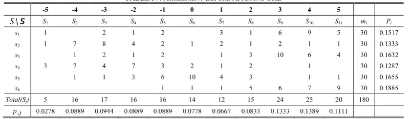
TABLEIV:AGREEMENT BEFORE APPLYING ORD
-5 -4 -3 -2 -1 0 1 2 3 4 5
S \ S S1 S2 S3 S4 S5 S6 S7 S8 S9 S10 S11 mi Pi
s1 1 2 1 2 3 1 6 9 5 30 0.1517
s2 1 7 8 4 2 1 2 1 2 1 1 30 0.1333
s3 1 2 1 2 1 3 10 6 4 30 0.1632
s4 3 7 4 7 3 2 1 2 1 30 0.1287
s5 1 1 3 6 10 4 3 1 1 30 0.1655
s6 1 1 1 5 6 7 9 30 0.1885
Total(Sj) 5 16 17 16 16 14 12 15 24 25 20 180
Thus, the proportion of all assignments, for instance, to category S11 is:
·,
1
,
1
180 5 1 1 9 0.1111
where 180. Then, we obtain
1
6 0.1517 0.1333 0.1885 0.1552
0.0278 0.0889 0.1111 0.1002
Finally, we obtain
0.1552 0.1002
1 0.1002 0.0610
Thus, from the above results, we can see
0.1289 0.0610 0.0679. That is, we obtain a 6.79% increase in the degree of agreement after applying our method. Note that the above 1 andM are the
normalization factors, which aredifferent from ones given in (1) and(3), respectively.
VII. CONCLUSION
This study explored a novel method for automatically detecting and removing outlying ratings.A series of basic concepts were introduced, which are used to characterise the ratingfrequency distributions and to establish rules for detecting and removing outliers. The key point of our method is that arating frequency is regarded as an outlier and removed if (i) it exhibits a very low frequency and/or,(ii) a high divergence from the mode. Our method was presented for samples with a single dominant category; it was alsoextended to samples with multiple dominant categories. The effectiveness of our method in improving thedegree of agreement between raters, assessed with the modified Fleiss' kappa, wasdemonstrated through a practical
example. It should be pointed out that the rating frequencydistributions of samples may be very complex and that the current study is pioneering work, so there remains a large gap to be filled for future work. Finally, we would expect ORD to bea useful tool in real world applications, in particular, involving web data gathering, ratingsand classification.
REFERENCES
[1] V. Barnett and T. Lewis, Outliers in Statistical Data, 3rd ed.: Wiley-Blackwell, 1994.
[2] I. B. Gal, “Outlier Detection,” in Data Mining and Knowledge Discovery Handbook: A Complete Guide for Practitioners and Researchers, O. Maimon and L. Rockach: Kluwer Academic Publishers, 2005, pp. 131-146.
[3] J. Dawes, “Do data characteristics change according to the number of scale points used?” International Journal of Market Research, vol. 50, no. 1, pp. 61-77, 2008.
[4] A. Donabedian, “The quality of care; how can it be assessed,” JAMA, vol. 260, no. 12, pp. 1743-1748, Sep. 1988.
[5] J. L. Fleiss, “Measuring nominal scale agreement among many raters,” Psychological Bulletin, vol. 76, no. 5, pp. 378-382, Nov. 1971. [6] F. E. Grubbs, “Procedures for detecting outlying observations in
samples,” Technometrics, vol. 11, no. 1, pp. 1-12, Nov. 1969. [7] T. Hu and S. Y. Sung, “Detecting pattern-based outliers,” Pattern
Recognition Letters, vol. 24, no. 16, pp. 3059-3068, Dec. 2003. [8] K. Krippendorff, Content Analysis: An Introduction to its
Methodology, Thousand Oaks, CA: Sage Publications, 2004. [9] D. S. Moore and G. P. McCabe, Introduction to the Practice of
Statistics: W. H. Freeman and Company, 1999.
[10] A. P. Morton and A.J. Dobson, “Analysing ordered categorical data from two independent samples,” British Medical Journal (BMJ), vol. 301, no. 6758, pp. 971-973, Oct. 1990.
[11] L. Moses, J. Emerson, and H. Hosseini, “Analysing data from ordered categories,” The New England Journal of Medicine, vol. 311, no. 7, pp. 442-448, 1984.
[12] J. Sim and C.C. Wright, “The kappa statistic in reliability studies: Use, interpretation, and sample size requirements,” Physical Therapy, vol. 85, no. 3, pp. 257-268, Mar. 2005.
[13] E. J. Snell, “A scaling procedure for ordered categorical data,” Biometrics, vol. 20, no. 3, pp. 592-607, Sep. 1964.
[14] M. Thelwall, K. Buckley, G. Paltoglou, D. Cai, and A. Kappas, “Sentiment strength detection in short informal text,” Journal of the American Society for Information Science and Technology, vol. 61, no. 12, pp. 2544-2558, Dec. 2010.
[15] J. A. Ting, A. D’Souza, and S. Schaal, “Automatic outlier detection: A Bayesian approach,” in IEEE International Conf. Robotics and Automation, 2007, pp. 2489-2494.
received her PhD in the Department of Computing Science at the University of Glasgow in UK. She is currently a research fellow in the School of Computing and Engineering at the University of Huddersfield in UK. Her main research interests include information extraction and retrieval, document classification and summarization, text mining and analytics, emotion and sentiment analysis. She is a member of the IEEE and ACM.
is a senior lecturer in Information Systems in the Department of Informatics at the University of Huddersfield in UK, where he has been since 1993. He teaches Web Programming and Database Development and has research interests in information retrieval and information systems development methods.
Di Cai