Journal of Engineering Sciences, Volume 6, Issue 2 (2019), pp. F 15–F 23 F 15 JOURNAL OF ENGINEERING SCIENCES
ЖУРНАЛ ІНЖЕНЕРНИХ НАУК
ЖУРНАЛ ИНЖЕНЕРНЫХ НАУК
Web site: http://jes.sumdu.edu.ua
DOI: 10.21272/jes.2019.6(2).f3 Volume 6, Issue 2 (2019)
Numerical Simulation of Viscous Dissipation and Chemical Reaction in MHD of Nanofluid
Govardhan K.1, Narender G.2*, Sarma G. S.2 1 GITAM University, Hyderabad, India; 2 CVR College of Engineering, Hyderabad, India
Article info:
Paper received:
The final version of the paper received: Paper accepted online:
May 4, 2019 August 26, 2019 August 31, 2019
*Corresponding Author’s Address:
[email protected]
Abstract. A study of viscous dissipation and chemical reaction effects of nanofluid flow passing over a stretched surface with the MHD stagnation point and the convective boundary condition has been analyzed numerically. The constitutive equations of the flow model are solved numerically and the impact of physical parameters concerning the flow model on dimensionless velocity, temperature and concentration are presented through graphs and tables. Also, a comparison of the obtained numerical results with the published results of W. Ibrahim has been made and found that both are in excellent agreement. As a result of the research, it was obtained that the magnetic parameter has the same increasing influence on the temperature and the concentration field but opposite on the velocity field, the tem-perature field, and the concentration field reduce with an increase in the Prandtl number, increase in viscous dissipa-tion increases temperature and concentradissipa-tion profile, and concentradissipa-tion as well as the thickness of concentradissipa-tion de-crease by increasing values of chemical reaction parameter.
Keywords: magnetohydrodynamic, stretching sheet, nanofluid, viscous dissipation, chemical reaction.
1
Introduction
During the past few years, investigating the stagnation point flow of nanofluids has become more popular among the researchers. Nanofluids are formed by the suspension of the nanoparticles in conventional base fluids. Exam-ples of such fluids are water, oil or other liquids. The nanoparticles conventionally made up of carbon nano-tubes, carbides, oxides or metals, are used in the nanoflu-ids. Keen interest has been taken by many researchers in the nanofluids as compared to the other fluids because of their significant role in the industry, medical field and a number of other useful areas of science and technology. Some prominent applications of these fluids are found in magnetic cell separation, paper production, glass blow-ing, cooling the electronic devices by the cooling pad during the excessive use, etc. Choi [1] introduced the idea of nanofluids for improving the heat transfer potential of conventional fluids. He experimentally concluded with evidence that injection of these particles helps in improv-ing the fluid's thermal conductivity. This conclusion opened the best approach to utilize such fluids in mechan-ical engineering, chemmechan-ical engineering, pharmaceutmechan-icals, and numerous different fields. Buongiorno [2], Kuz-netsov and Nield [3] followed him and extended the in-vestigation. They worked on the effects of Brownian motion in convective transport of nanofluids and the
in-vestigation of natural convective transport of nanofluids passing over a vertical surface in a situation when nano-particles are dynamically controlled at the boundary. Khan and Pop [4] used this concept to evaluate the lami-nar boundary layer flow, nanoparticles fraction and heat transfer for nanofluids passing over a stretching surface.
2
Literature Review
F 16 CHEMICAL ENGINEERING: Processes in Machines and Devices Naramgari and Sulochana [7] outlined the mass and
heat transfer of the thermophoretic fluid flow past an exponentially stretched surface inserted in porous media in the presence of internal heat generation/absorption, infusion, and viscous dissemination. Afify [8] examined the MHD free convective heat and fluid flow passing over the stretched surface with chemical reaction. A nu-merical analysis of insecure MHD boundary layer flow of a nanofluid past a stretched surface in a porous media was carried out by Anwar et al. [9]. Nadeem and Haq [10] studied the magnetohydrodynamic boundary layer flow with the effect of thermal radiation over a stretching surface with the convective boundary conditions.
Our prime objective is, we first reproduce an analysis study of [11] and then extend the MHD stagnation point flow of nanofluid past a stretching sheet with convective boundary condition. According to our information, vis-cous dissipation and chemical reaction effects on MHD mixed convection stagnation point flow of nanofluid over a stretching surface is not yet examined. An appropriate similarity transformation has been utilized to acquire the system of nonlinear and coupled ODEs from the system of PDEs. Results are acquired numerically by using the comprehensive shooting scheme. The numerical results are analyzed by graphs for different parameters which appear in the solution affecting the MHD mixed convec-tion stagnaconvec-tion point.
3
Research Methodology
3.1
Mathematical Modeling
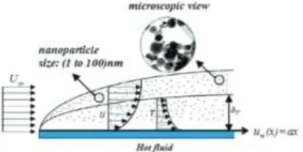
Consider the stagnation point flow of two-dimensional viscous steady flow of nanofluid passing over a stretched surface with the convective boundary condition (BC). The stretching sheet was heated with the temperature Tf
and the heat transfer coefficient hf at its lower surface.
Here, concentration and uniform ambient temperature are respectively C∞ and T∞.
Assume that at the surface, there is not any nanoparti-cle flux and the impacts of the thermophoresis are taken as a BC. In flow model, uw(x) = ax is the velocity of the
stretching surface, where “a” is any constant. In the direc-tion of the flow, normal to the surface, it is directed to-wards the magnetic field of strength B0 which is supposed to be applied in the direction of + ve y-axis. Here magnetic field is negligible because of as-sumption of very small when compared with the applied magnetic field. The preferred system of coordinates is such as x-axis is directed to the flow and y-axis is per-pendicular to it. Proposed coordinate system and flow model are presented in Figure 1.
Flow model of W. Ibrahim [11] shows that in the pres-ence of magnetic field over the surface, the governing equations of conservation of momentum, energy, mass and nanoparticle fraction, under the boundary layer ap-proximation, are as follows:
(1)
Figure 1 – Geometry for the flow under consideration
(2)
(3)
(4)
The associated boundary conditions are:
(5)
where x is the coordinate axis along the continuous surface in the direction of motion and y is the coordinate axis along the continuous surface in the direction perpen-dicular to the motion. The components of velocity along x- and y-axis are respectively u and v. Here kinematic velocity is represented by ν and T represents the tempera-ture inside the boundary layer. The parameter τ is defined by τ = (ρc)p/(ρc)f , where (ρc)p is effective heat capacity
of nanoparticles and (ρc)f is heat capacity of the base
fluid, ρ is the density and T∞ is the ambient temperature far away from the surface.
The radiative heat flux qr is given as
(6)
where σ* and k* stand for the Stefan-Boltzmann con-stant and coefficient of mean absorption, and T 4 is the linear sum of temperature and it can expand with the help of Taylor series along with T∞
(7) ignoring higher order terms, we get
Journal of Engineering Sciences, Volume 6, Issue 2 (2019), pp. F 15–F 23 F 17 substituting (8) into (6), we get
(9)
To convert the PDEs (1)–(4) along with the BCs (5) into the dimensionless form, we use the similarity trans-formation [11]:
, . (10)
In above, ψ(x, y) denotes stream function obeying
(11)
The equation of continuity (1) is satisfied identically, the effect of stream function on the remaining three tions, the momentum equation (2), the temperature equa-tion (3) and concentraequa-tion equaequa-tion (4) are
(12)
(13) (14)
The BCs get the form:
at (15) as (16) In equations (12)–(14), the governing parameters are defined as is the radiation parameter, , is Prandtl number, is Lewis number, is a magnetic parameter, is
veloc-ity ratio parameter, is
Brown-ian motion parameter,
thermophoresis parameter, Biot number, is the Eckert number and is the chemical reaction parameter. In this problem, the desired physical quantities are the local Nusselt number Nux, and reduced Sherwood number
Shx and the skin-friction coefficient Cf. These quantities
are defined as
,
(17)
Here, τw is the shear stress along the stretching surface, qw is the heat flux from the stretching surface and hw is
the wall mass flux, are given as
(18)
With the help of the above equations, we get
(19)
where Rx = ax2 is the local Reynolds number.
3.2
Numerical calculations
The analytic solution of the system of equations with corresponding boundary conditions (12)–(14) cannot be found because they are nonlinear and coupled. So, we use numerical technique, i. e., shooting–Newton technique with fourth-order Adam’s–Moultan method. In order to solve the system of ordinary differential equations (12)– (14) with boundary conditions (15), (16) using shooting method, we have to convert these equations into a system of first-order differential equations, let
(20)
Then the coupled nonlinear momentum, temperature and concentration equations are converted into system of seven first-order simultaneous equations and the corre-sponding boundary conditions transform the following form:
, , , ,
, , (21)
/(1+R),
, , t,
, +
,
The above equations (21) are solved using Adam’s– Moultan method of order 4 with an initial guess
. These guesses are updated by Newton’s method. The iterative process is repeated until the follow-ing criteria is
where ϵ > 0 is tolerance.
For all computation in this paper, we have fixed ϵ =10– 5. The step sizes of Δ𝜂 = 0.01 and η
max = 10 were found to
F 18 CHEMICAL ENGINEERING: Processes in Machines and Devices
4
Results
The objective of this section is to analyze the numeri-cal results displayed in the shape of graphs and tables. The computations are carried out for various values of the magnetic parameter M, velocity ratio parameter A, radia-tion parameter Nr, Eckert number Ec, Lewis number Le, Brownian motion parameter Nb, thermophoresis parame-ter Nt and Prandtl number Pr, and the impact of these parameters on the velocity, temperature, and concentra-tion profiles are also discussed in detail.
Table 1 shows the comparison of calculated values with [11, 12] and strong agreement with the values is found which showed high confidence of present simula-tion. In Table 1, by taking M = 0 and update the velocity ratio parameter A, numerical results of the skin-friction coefficient –f''(0) are reproduced.
Table 1 – Comparison of the skin-friction coefficient –f''(0) for different values of velocity ratio parameter A and M = 0
A Ibrahim [11], Ishak [12] Present result
0.1 −0.9694 –0.9693874
0.2 −0.9181 –0.9181041
0.3 −0.8494 –0.8494202
0.4 −0.7653 –0.7653250
0.5 −0.6673 –0.6672632
0.8 −0.2994 –0.2993885
1.0 0.0000 0.0000000
2.0 2.0175 2.0175020
3.0 4.7293 4.7292940
5.0 11.7520 11.7519900
7.0 20.4979 20.4980600
10.0 36.2574 36.2575000
To further investigate the numerical technique used, by ignoring the impacts of thermophoresis parameter Nt and Brownian motion parameter Nb and then compare the local Nusselt number –θ'(0) by updating the Prandtl number as shown in Table 2. Excellent agreement of current results with those previously published results encourages us to use the present code.
Table 2 – Comparison of the local Nusselt number –θ'(0) when Nt = 0 and Nb → 0 for different values of Pr
Pr A Present result Ibrahim [11] Mahapatra [13] Hayat [14] 1.0 0.1 0.6008148 0.6028 0.603 0.602156 1.0 0.2 0.6246567 0.6246 0.625 0.624467 1.0 0.3 0.6926060 0.6924 0.692 0.692460 1.5 0.4 0.7760525 0.7768 0.777 0.776802 1.5 0.5 0.7969141 0.7971 0.797 0.797122 1.5 0.8 0.8648634 0.8648 0.863 0.864771 2.0 1.0 0.9256601 0.9257 – – 2.0 2.0 0.9447336 0.9447 – – 2.0 3.0 1.0114910 1.0116 – –
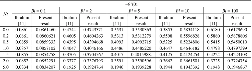
Furthermore, we reproduce the results of [11] for the local Nusselt number –θ '(0). Table 3 presents the local Nusselt number –θ '(0) by taking random values of dif-ferent physical parameters used such as Brownian mo-tion, thermophoresis parameter, Biot number, and the velocity ratio. It is observed in the table that the local Nusselt number –θ '(0) is decreasing function of the thermophoresis parameter Nt and an increasing function of the Biot number Bi.
Table 3 – Comparison of the local Nusselt number –θ '(0) for the different values of Nt and Bi if Nb = 5, A = 0.3, Pr = M = 1, Le = 5
Nt
–θ '(0)
Bi = 0.1 Bi = 2 Bi = 5 Bi = 10 Bi = 100
Ibrahim [11] Present result Ibrahim [11] Present result Ibrahim [11] Present result Ibrahim [11] Present result Ibrahim [11] Present result 0.0 0.0861 0.0861460 0.4744 0.4743371 0.5531 0.5530363 0.5855 0.5854118 0.6180 0.6179690 0.2 0.0861 0.0860621 0.4605 0.4604263 0.5313 0.5312279 0.5598 0.5596828 0.5880 0.5878806 0.5 0.0859 0.0859333 0.4395 0.4394668 0.4993 0.4992715 0.5225 0.5224806 0.5415 0.5450010 1.0 0.0857 0.0857102 0.4047 0.4046166 0.4486 0.4485220 0.4647 0.4646182 0.4798 0.4797399 1.5 0.0855 0.0854758 0.3705 0.3704567 0.4017 0.4015988. 0.4125 0.4124254 0.4224 0.4223108 2.0 0.0852 0.0852291 0.3377 0.3376793 0.3591 0.3590596 0.3662 0.3661501 0.3725 0.3724754 5.0 0.0834 0.0834207 0.1925 0.1924764 0.1940 0.1939228 0.1944 0.1943392 0.1948 0.1946867
Figure 2 divulges the impact of the magnetic parame-ter on the velocity f '(0). Here, due to magnetic field, an opposing force which is called Lorentz force appears which resist the flow of fluid and consequently the flow of velocity declines.
Figure 3 designates the impact of Pr on the tempera-ture profile θ(η). It is clear from the figure that the tem-perature of the flow field is the decreasing function of Pr. It is because of the way when Pr of fluid is high then thermal diffusion is low if it is compared with the viscous
diffusion. Consequently, the coefficient of heat transfer declines as well as shrinks the thickness of the boundary layer.
Journal of Engineering Sciences, Volume 6, Issue 2 (2019), pp. F 15–F 23 F 19 Figure 5 describes the effect of the convective heating
which is also known as the Biot number on the tempera-ture profile θ(η). Numerically, it can be calculated by dividing the convection on the surface to the conduction into the surface of an object. When Bi increases, it causes an increase in the temperature on surface which sequels in the thickening of the thermal boundary layer.
The effect of velocity ratio parameter A on the temper-ature profile θ(η) has been highlighted in Figure 6. As we increase the value of velocity ratio parameter A, the tem-perature at the surface declines, and furthermore, it also declines the thickness of the thermal boundary layer.
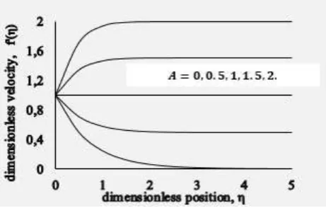
Figure 2 – Velocity profile f '(0) for different values of velocity ratio A, when Pr = 1.0, Nr = 3, Ec = 1.0, kc = 1.0, Nt = 0.5,
Nb = 0.5, Le = Bi = 5.0, M = 1.0
Figure 3 – Velocity profile f '(0) for different values of M when Pr = 1.0, Nr = 3, Ec = 1.0, kc =1.0, Nt = 0.5, Nb = 0.5,
Le = Bi = 5.0
Figure 4 – Variation of θ(η) for various values of Pr when M = 1.0, A = Nt = Nb = 0.5, Bi = Le = 5.0,
Ec = Nr = 0, and kc = 1.0
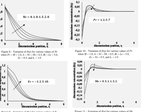
The influence of radiation parameter on the profile of temperature distribution is displayed in Figure 7. Tem-perature increases with the increase of thermal radiation parameter Nr. The effect of radiation intensifies the heat transfer thus radiation should be at its minimum in order to facilitate the cooling process.
Figures 8 show the impact of the viscous dissipation on the temperature profile. When the value of the viscous dissipation is increased, the fluid region is allowed to store the energy. As a result of dissipation due to friction-al heating, heat is generated.
Figure 5 – Variation of θ(η) for various values of Nt when Pr = M = 1.0, A = Nb = 0.5, Le = 5.0,
Ec = Nr = 0.5, and kc = 1.0
Figure 6 – Variation of θ(η) for various values of Bi when Pr = M = 1.0, A = Nt = Nb = 0.5, Le = 5.0,
Ec = Nr = 0.5, and kc = 1.0
Figure 7 – Variation of θ(η) for various values of A when Pr = M = 1.0, Nt = Nb = 0.5, Le = 5.0,
F 20 CHEMICAL ENGINEERING: Processes in Machines and Devices The effect of the variation in the Pr on the
concentra-tion profile is observed in Figure 9. It is noticed from the figure, as the value of Prandtl number rises, the nanopar-ticles scattered out toward the outward, consequently, the nanoparticles concentration at the surface decreases.
The impact of the Brownian motion parameter Nb on the concentration β(η) is illustrated in Figure 10. When we increase the effect of Nb, the concentration profile β(η) also increases initially but it starts decreasing far away from the wall.
It seems clear from the Figure 11 that if we increase the thermophoretic force, it causes decline in the concen-tration profile β(η) at the surface, which is reverse in nature to the case of the Nt.
The concentration vs Lewis number has been illustrat-ed in Figure 12. Increasing Le corresponding to the con-centration. As a result, initially the concentration on face increases but after a while, a bit away from the sur-face it starts decreasing.
Figure 8 – Variation of θ(η) for various values of Nr when Pr = M = 1.0, A = Nt = Nb = 0.5, Bi = Le = 5.0,
Ec = 0.5, and kc = 1.0
Figure 9 – Variation of θ(η) for various values of Ec when Pr = M = 1.0, A = Nt = Nb = 0.5, Bi = Le = 5.0,
Nr = 0.5, and kc = 1.0
Figures 13 and 14 demonstrate the concentration vs velocity ratio. It has similar effects on the concentration profile as the effect of the Lewis number is noted on con-centration. As the concentration distribution decreases by increasing the velocity ratio parameter A.
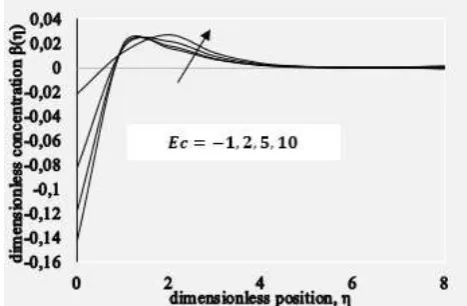
Figure 15 display the influence of Eckert number Ec on the concentration profile. It is observed that the con-centration of the fluid decreases near the plate. However, it rises away from the surface as the value of Eckert num-ber is enhanced.
Figure 16 explains the influence of the chemical reac-tion parameter on the profile of concentrareac-tion. It is noted that increasing values of chemical reaction parameter concentration as well as the thickness of concentration decrease. It is because of the fact that the chemical reac-tion in this system results in chemical dissipareac-tion and therefore results in a decrease in the profile of concentra-tion. The most significant influence is that chemical reac-tion tends to increase the overshoot in the concentrareac-tion profiles and their associated boundary layer.
Figure 10 – Variation of β(η) for various values of Pr when M = 1.0, A = Nt = Nb = 0.5, Bi = Le = 5.0,
Ec = Nr = 0.5, and kc = 1.0
Figure 11 – Variation of β(η) for various values of Nb when Pr = M = 1.0, A = Nt = 0.5, Bi = Le = 5.0,
Journal of Engineering Sciences, Volume 6, Issue 2 (2019), pp. F 15–F 23 F 21 Figure 12 – Variation of β(η) for various values of Nt
when Pr = M = 1.0, A = Nb = 0.5, Bi = Le = 5.0, Ec = Nr = 0.5, and kc = 1.0
Figure 13 – Variation of β(η) for various values of Le when Pr = M = 1.0, A = Nt = Nb = 0.5, Bi = 5.0,
Ec = Nr = 0.5, and kc = 1.0
Figure 14 – Variation of β(η) for various values of A when Pr = M = 1.0, Nt = Nb = 0.5, Bi = Le = 5.0,
Ec = Nr = 0.5, and kc = 1.0
Figure 15 – Variation of β(η) for various values of Ec when Pr = M = 1.0, A = Nt = Nb = 0.5, Bi = Le = 5.0,
Nr = 0.5, and kc = 1.0
Figure 16 – Variation of β(η) for various values of kc
when Pr = M = 1.0, A = Nt = Nb = 0.5, Bi = Le = 5.0, Nr = 0.5, and Ec = 1.0
5
Conclusions
After a thorough investigation, we have reached the concluding observation. Particularly, the velocity profile increases by increasing the parameter A, but the tempera-ture and concentration profiles decrease by increasing this parameter. The magnetic parameter M has the same in-creasing influence on the temperature and the concentra-tion field but opposite on the velocity field. The tempera-ture field θ(η) and the concentration field β(η) reduce with an increase in the Prandtl number. Temperature field θ(η) increases with an increase in thermal radiation Nr.
For larger values of Lewis number Le, thermophoresis parameter Nt, and Brownian motion parameter Nb has an increasing effect on the concentration field β(η).
F 22 CHEMICAL ENGINEERING: Processes in Machines and Devices
6
Acknowledgments
The authors would like to thanks to Prof. Koneru S. R., Retired Professor, Department of Mathematics, Indian Institute of Technology Bombay for his support through-out this research work.
7
Nomenclature
magnetic field strength Constant
Brownian diffusion coefficient thermophoretic diffusion coefficient thermal conductivity
Stefan-Boltzmann constant mean absorption
Eckert number Lewis number magnetic parameter
Brownian motion parameter thermophoresis parameter Nusselt number
reduced Nusselt number Prandtl number
pressure
heat capacity of the fluid
effective heat capacity of the nanoparticle mate-rial
radiative heat flux
wall mass flux wall heat flux
local Reynolds number reduced Sherwood number local Sherwood number fluid temperature
the temperature at the stretching sheet ambient temperature
velocity components along and axis the velocity of the stretching sheet
Cartesian coordinates ( axis is aligned along the stretching surface and axis is normal to it)
thermal diffusivity
dimensionless nanoparticle volume fraction similarity variable
stream function
dimensionless temperature fluid density
nanoparticle mass density
the electrical conductivity of the fluid parameter defined by the ratio between the ef-fective heat capacity of the nanoparticle materi-al and heat capacity of the
flu-id.
References
1. Choi, S. (1995). Enhancing thermal conductivity of fluids with nanoparticles. ASME-Publications-Fed, Vol. 231, pp. 99–106. 2. Buongiorno, J. (2006). Convective transport in nanofluids. Journal of Heat Transfer, Vol. 128(3), pp. 240–250.
3. Kuznetsov, K. V., Nield, D. A. (2010). Natural convective boundary-layer flow of a nanofluid past a vertical plate. International Journal of Thermal Sciences, Vol. 49(2), pp. 243–247.
4. Khan, W. A., Pop, I. (2011). Flow and heat transfer over a continuously moving at plate in a porous medium. Journal of Heat Transfer, Vol. 133(5), art. no. 054501.
5. Makinde, O. D., Khan, W. A., Khan, Z. H. (2013). Buoyancy effects on MHD stagnation point flow and heat transfer of a nanofluid past a convectively heated stretching/shrinking sheet. International Journal of Heat and Mass Transfer, Vol. 62, pp. 526–533.
6. Cortell, R. (2012). Heat transfer in a fluid through a porous medium over a permeable stretching surface with thermal radiation and variable thermal conductivity. The Canadian Journal of Chemical Engineering, Vol. 90(5), pp. 1347–1355.
7. Naramgari, S., Sulochana, C. (2016). Dual solutions of radiative MHD nanofluid flow over an exponentially stretching sheet with heat generation/absorption. Applied Nanoscience, Vol. 6(1), pp. 131–139.
8. Afify, A. A. (2004). MHD free convective flow and mass transfer over a stretching sheet with chemical reaction. Heat and Mass Transfer, Vol. 40(6–7), pp. 495–500.
9. Beg, O. A., Khan, M. D. S., Karim, I., Alam, M. D. M., Ferdows, M. (2014). Explicit numerical study of unsteady hydromagnet-ic mixed convective nanofluid flow from an exponentially stretching sheet in porous media. Applied Nanoscience, Vol. 4(8), pp. 943–957.
10. Nadeem, S., Haq, R. U. (2014). Effect of thermal radiation for magnetohydrodynamic boundary layer flow of a nanofluid past a stretching sheet with convective boundary conditions. Journal of Computational and Theoretical Nanoscience, Vol. 11(1), pp. 32–40.
Journal of Engineering Sciences, Volume 6, Issue 2 (2019), pp. F 15–F 23 F 23 12. Ishak, A., Nazar, R., Pop, I. (2006). Mixed convection boundary layers in the stagnation point flow toward a stretching vertical
sheet. Meccanica, Vol. 41(5), pp. 509–518.
13. Mahapatra, T. R., Gupta, A. S. (2002). Heat transfer in stagnation-point flow towards a stretching sheet. Heat and Mass Transfer, Vol. 38(6), pp. 517–521.
14. Hayat, T., Mustafa, M., Shehzad, S. A., Obaidat, S. (2012). Melting heat transfer in the stagnation-point flow of an upper convected Maxwell (UCM) fluid past a stretching sheet. International Journal for Numerical Methods in Fluids, Vol. 68, art. no. 233243.
УДК 537.84
Числове дослідження в’язкої дисипації та хімічної реакції
у магнітогідродинаміці нанорідини
Говардхан К.1, Нарендер Г.2, Сарма Г. С.2
1 Університет технологій та управління ім. Ганді, м. Гайдарабад, Індія; 2 Інженерний коледж CVR, м. Гайдарабад, Індія
Анотація. У роботі розглядається числове дослідження впливу в’язкої дисипації та хімічної реакції потоку нанорідини, що проходить через натягнуту поверхню з магнітогідродинамічною зоною застою для заданих граничних умов. Основні рівняння моделі потоку розв’язуються чисельно. Вплив фізичних параметрів мате-матичної моделі потоку на безрозмірну швидкість, температуру і концентрацію подано із застосуванням від-повідних графіків і таблиць. Також було проведено порівняння отриманих числових результатів з опубліко-ваними результатами. У результаті встановлено, що результати узгоджуються із високою точністю. Також було отримано, що магнітний параметр має однаковий вплив на температуру і поле концентрації. Проте на-впаки, вплив на поля швидкості, температури і концентрації зменшується зі збільшенням числа Прандтля. Також збільшення в’язкої дисипації збільшує температуру і концентрацію, а також товщина шару зменшу-ється за рахунок збільшення значень параметра хімічної реакції.